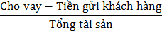
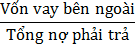
Regression Results of Factors Affecting Rrtk at Agribank (Dependent Variable: Fgapr)

In which, external loans include debts from the State Bank, loans from other credit institutions and issuance of valuable papers and this indicator has a unit of %.

Dependence on external funding sources and RRTK have positive effects.

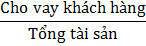
- Customer Loan to Value Ratio (TLA)

In Vietnam as well as some other countries, the most traditional and important activity of banks is still lending. However, according to Bonfim and Kim (2008), conventional loans, especially retail loans, are not highly liquid, so large unforeseen withdrawals can cause liquidity risk for banks [83]. Therefore, in the scope of this study, customer loans will be used because these loans are often low in liquidity. Therefore, the author expects a positive relationship between the customer loan ratio and liquidity risk.

The loan rate is expressed in % and is calculated using the following formula:

- Return on equity (ROE)

This ratio is measured by dividing profit after tax by total equity, so it reflects the bank's management efficiency in using equity. Most previous studies use the ratio of Profit after tax/Total assets to assess the bank's liquidity. Some studies found a positive impact of profit ratio on bank liquidity (Bonfim and Kim, 2008) [83]. But some studies also found an inverse impact of profit ratio on RRTK (Vodová, 2011) [129]. These studies use the ROE ratio because on the one hand they want to assess the ability to use equity, and on the other hand they want to consider the impact of this factor on the bank's RRTK.

The net profit to equity ratio will have a positive impact on the RRTK of bank branches.

Return on equity is expressed in % and has the following formula:

b. Objective factors

- Economic growth rate (GDP)

GDP is the monetary value of all final goods and services produced within an economy in a given period of time (usually a fiscal year). The GDP growth rate is calculated as follows.

In which: GDP is GDP growth rate (%) GDP t is GDP of year t

GDP t-1 is the GDP of year (t-1)

There is a positive relationship between GDP growth rate and RRT.

- Inflation rate (CPI)

In economics, inflation is an increase over time in the general price level of the economy. The general price level is the average price of many goods and services and is measured by price indexes, which are indicators reflecting the price level at a certain point in time as a percentage of the previous point in time or the base point. There are many ways to calculate the inflation index. The thesis uses the consumer price index CPI. The calculation formula is as follows:

In which: CPI is the inflation rate (%) CPI t is the consumer price index of year t

CPI t-1 is the consumer price index of year (t-1).

This is the most common way of calculating inflation in the world and is also the standard that the National Assembly uses to measure the inflation rate under the 2010 Law on the State Bank of Vietnam.

Inflation rate and RRTK have a positive relationship.

- Money supply growth (M2)

The money supply velocity must be equal to the GDP growth rate, a quantity of money supply

Excessive money supply can be a source of inflation. Changes in the money supply, through various central bank tools, can affect bank liquidity. An expansionary monetary policy can increase bank liquidity.

The formula for calculating the inflation rate change is as follows:

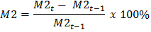
In which: M 2 is the change in money supply (%) M 2t is the money supply of year t

M 2t-1 money supply of year (t-1).

There is an inverse relationship between M2 and bank liquidity.

The dependent and independent variables in the model are summarized below.

Table 2.19: Explanation of variables in the model

Factor

Symbol	Explain	Expectation Sign
Dependent variable
Funding gap ratio	FGAPR
Independent variable
Dependence on external capital	EFD		+
Customer loan ratio	TLA		+
Return on equity	ROE		+
Economic growth rate	GDP		+
Inflation rate	CPI		+
Money supply growth	M 2		-

Maybe you are interested!

2.2.2.3. Analysis method

The thesis uses panel data analysis method with data series changing over time (6 years, from 2011-2016) and space (25 branches of Agribank). Currently, there are 3 popular panel data approaches: Pooled OLS,

FEM and REM. Pooled OLS is a panel data approach that stacks all observations together, ignoring the spatial and temporal dimensions and estimating only using the ordinary OLS model, so the regression coefficients are and are assumed to be the same for all observations. Meanwhile, FEM helps to separate the effects of individual characteristics from the independent variables to estimate the real effects of the independent variables on the dependent variable. This means that when considering the effects of space and time, the intercepts will change differently for each branch. However, because the data series used in the study is short in time, using this approach can also cause the model's estimates to be biased. The thesis does not use REM because this approach assumes that the individual characteristics between branches are assumed to be random. In addition, the REM model may lack variables, so it can produce inaccurate estimation results.

While Chung (2009) used the FEM model to explain the results, due to the limitations of the model, this thesis will regress all three models Pooled OLS, FEM and REM - then test the appropriateness between the Pooled OLS model and the REM model based on the Breusch-Pagan test with the hypothesis:

Ho: Panel data effect does not exist (Pooled OLS model is efficient) H 1 : Panel data effect exists (i.e. REM model is efficient)

Next, to evaluate the fit between the two FEM and REM models, the study

The study will use the Hausman test to examine whether there is any correlation between the explanatory variables and the random components. The hypothesis is:

Ho: There is no correlation between the independent variables and the random component H 1 : There is a correlation between the explanatory variables and the random component If the obtained P-value is greater than the 5% significance level, there is not enough basis to reject the hypothesis.

Ho hypothesis, according to which REM model will be selected. In the opposite situation, FEM model will be used.

In the case of the most optimal model in the trio Pooled OLS, FEM and REM still has some limitations such as autocorrelation or heteroscedasticity leading to instability, the Generalized dynamic array data analysis method

Method of Moment (GMM) will be applied to test the above relationship. The biggest advantage of the GMM method compared to the conventional OLS estimation method, FEM fixed effect estimation and REM random effect estimation is that it has solved the problem of omitted endogenous variables and measurement errors in the regression process.

Arif and Anees (2012) study shows that clearly distinguishing the endogenous variable group (lagged variables that have a causal relationship with the dependent variable - the regression of these variables will lead to correlation with the error, that is, the endogenous phenomenon biases the results) and the instrumental variable group (including strictly exogenous variables and additional instrumental variables with appropriate lags) is the most important step in the GMM procedure, determining the quality of the estimation [63]. Performing first-order differences on both sides of the linear equation, the study obtained the general form of the GMM equation as follows:

ΔY it = α' ΔY i,t-1 + β' ΔX i,t-1 + γ' Z it + Δu i (*)

In there:

ΔY it and ΔY i,t-1 are the first difference and first difference lag of the dependent variable,

ΔX i,t-1 is the first-difference lag of the endogenous variable, Z it represents the group of exogenous variables.

The suitability of the instrumental variables used in GMM regression is assessed based on the Hansen test (overidentifying restrictions), with the hypothesis (H 0 ): The instrumental variables are exogenous, meaning they are not correlated with the model error. Therefore, the larger the p-value of the Hansen statistic, the better. Meanwhile, the larger the p-value of the AR(2) test result, the more it proves that the model does not have autocorrelation defects at all levels. In addition, in order for these tests to not be weak, the principle that the number of instrumental variables is less than or equal to the number of groups must be ensured. Finally, to argue that the results of the GMM model are good enough - to ensure robustness, the coefficient signs corresponding to each explanatory variable in the GMM model and in the fixed-effects regression model (FEM) or random-effects regression model (REM) must be consistent [123].

2.2.2.4. Data collection

The system of variables used in the model includes macroeconomic variables and internal bank variables. The variables belonging to the objective factor group include GDP growth rate (%), inflation rate (%) and M2 money supply growth rate in the period 2011-2016, which were studied and synthesized from the Worldbank website and data reports of the General Statistics Office.

The group of subjective factors affecting FGAPR liquidity risk was synthesized by the author from the audited financial statements of 25 branches of Agribank nationwide in the period 2011-2016 5 . In general, the scale of many Agribank branches is quite large, possibly equivalent to the scale of some domestic commercial banks. The calculation of indicators to serve the research topic was synthesized from Agribank's financial statements. The data source for quantitative research within the scope of the thesis is reliable.

2.2.2.5. Model results

a. Descriptive statistics of variables

Panel data (annual frequency) for the model running process includes 7 variables, 150 observations studied in the period 2011-2016.

Table 2.20: Descriptive statistics of variables in the model

Variable

Medium	Standard deviation	Min	Max
FGAPR	27.26	462.42	-63.64	57.43
EFD	3.96	9.38	0.36	69.67
TLA	61.30	6,682	13.57	81,911
ROE	12.61	9.50	-29.42	56.86
GDP	5.10	0.85	4.12	6.68
CPI	7.35	5.67	0.88	18.68
M2	18.50	4.14	11.94	24.54

Source: Author's calculation

(i) The dependent variable FGAPR has an average value of 27.26%, the smallest value is -63.64% and the largest is 57.43%, the standard deviation is quite high, reaching 462.42%. This shows that RRTK is very diverse and has a high difference between branches across the years.

5 Branches: Transaction Office, Lang Ha, Hanoi, Da Nang, Ha Tay, Hai Duong, Hung Yen, Bac Giang, Bac Ninh, Phu Tho, Nam Dinh, Thai Binh, Thanh Hoa, Ha Tinh, Quang Nam, Binh Thuan, Lam Dong, Binh Duong, Tay Ninh, Dong Nai, Long An, Tien Giang, Quang Ninh, Thai Nguyen, Nghe An.

year, from there, each Branch must have its own risk management strategy to be able to develop stably and sustainably.

(ii) The average external debt ratio (EFD) in the period 2011-2016 reached 3.96%, the standard deviation was moderate (9.38%), showing that different branches have very different levels of dependence on external debt ratio. The smallest value of 0.36% was achieved at Ha Tinh branch in 2012, and the largest value of 69.67% was achieved at So Giao Dich branch in 2016.

(iii) The customer loan to value ratio (TLA) has a fairly low standard deviation (6.68%). The lowest TLA of 13.57% was recorded at Lang Ha branch in 2014, while the highest of 81.9% was achieved at Phu Tho branch in 2014. The average TLA for the whole period reached 61.3%.

(iv) Return on equity (ROE) reached its lowest value (-29.42%) at the Quang Ninh branch in 2015, and its highest value was 56.86% at the Hanoi branch in 2012, with the average for the entire period recording 12.61%. The standard deviation of ROE of banks was moderate, 9.5%.

(v) Average GDP growth reached 5.1% and tended to be stable over the years, as shown by the lowest standard deviation of all variables at 0.85%. The lowest growth value of 4.12% was achieved in 2012 and the highest was 6.68% in 2016.

(vi) The inflation rate has a very large difference between the maximum and minimum values: the minimum value of 0.88% was achieved in 2015 as a result of the SBV's inflation control policy and the maximum value reached 18.68% in 2010 due to the impact of hot credit growth in the period 2007-2008. Accordingly, the average inflation rate for the whole period reached 7.35% and the standard deviation was 5.67%.

(vii) The average M2 growth rate over the period reached 18.5%, showing high stability over the years similar to GDP (low standard deviation: 4.14%). The lowest M2 growth rate of 11.94% was achieved in 2011, while the highest was 24.54% in 2012.

The correlation trend between the funding gap ratio and the explanatory factors coincides quite well with the hypothesis of the expected correlation sign as stated in the previous section. The pairwise correlation level between the independent variables is lower than 0.5, indicating the problem of multicollinearity.

The line in the model is not of concern [106].

Table 2.21: Correlation matrix between variables

FGAPR	EFD	TLA	ROE	GDP	CPI	M2
FGAPR	1
EFD	-0.020	1
TLA	0.999	-0.019	1
ROE	-0.169	0.034	-0.147	1
GDP	-0.033	-0.014	-0.024	0.178	1
CPI	-0.032	0.074	-0.047	-0.189	-0.244	1
M2	0.021	-0.027	0.025	0.051	-0.487	-0.334	1

Source: Author's calculation

b. Results and discussion

The study will regress the Pooled OLS, FEM and REM models in turn. The Breusch-Pagan test will then be performed to assess the suitability between the Pooled OLS and REM models, and finally the Hausman test to select the most optimal model between FEM or REM will be performed. To assess the level of model defects, tests on autocorrelation and heteroscedasticity will also be conducted. The regression results of factors affecting RRTK at Agribank are presented in the table below.

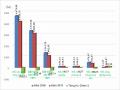
Table 2.22: Regression results of factors affecting RRTK at Agribank (Dependent variable: FGAPR)

Pooled OLS	REM	FEM	GMM*
FGAPR (-1)	-	-	-	0.004 0.006
EFD (-1)	-0.026 (0.183)	0.331** (0.165)	0.403** (0.176)	2,019*** (0.504)
TLA	0.069*** (0.000)	0.069*** (0.000)	0.069*** (0.000)	0.069*** (0.001)
ROE	-0.937*** (0.159)	-0.469*** (0.101)	-0.438*** (0.103)	-1.636*** (0.463)
GDP (-1)	-1,968 (3,788)	-2,843* (1,470)	-2,918** (1,435)	-0.565*** (3.857)
CPI	3,634 (3,557)	2,902** (1,383)	2,895** (1,350)	5,535*** (1,954)
M 2	-2,115 (3,058)	-1,428 (1,194)	-1,427 (1,166)	-4,047 (2,059)
Constant	27,957 (56,221)	14,679 (22,091)	14,354 (21,373)	-

Comment