Table 4.3: KMO and Bartlett's Test for the scale of independent variables KMO and Bartlett's Test
KMO coefficient
0.710 | ||
Bartlett test model | Chi-Square Value | 1193.272 |
Degrees of freedom | 190 | |
Sig (p – value) | .000 |
Maybe you are interested!
-

 Kmo Test and Bartlett's Test for Independent Variables
 -
 Kmo Coefficient And Bartlett'S Scale Component
 -
![Mobile Phone Usage in Hanoi Inner City Area
zt2i3t4l5ee
zt2a3gsconsumer,consumption,consumer behavior,marketing,mobile marketing
zt2a3ge
zc2o3n4t5e6n7ts
- Test the relationship between demographic variables and consumer behavior for Mobile Marketing activities
The analysis method used is the Chi-square test (χ2), with statistical hypotheses H0 and H1 and significance level α = 0.05. In case the P index (p-value) or Sig. index in SPSS has a value less than or equal to the significance level α, the hypothesis H0 is rejected and vice versa. With this testing procedure, the study can evaluate the difference in behavioral trends between demographic groups.
CHAPTER 4
RESEARCH RESULTS
During two months, 1,100 survey questionnaires were distributed to mobile phone users in the inner city of Hanoi using various methods such as direct interviews, sending via email or using questionnaires designed on the Internet. At the end of the survey, after checking and eliminating erroneous questionnaires, the study collected 858 complete questionnaires, equivalent to a rate of about 78%. In addition, the research subjects of the thesis are only people who are using mobile phones, so people who do not use mobile phones are not within the scope of the thesis, therefore, the questionnaires with the option of not using mobile phones were excluded from the scope of analysis. The number of suitable survey questionnaires included in the statistical analysis was 835.
4.1 Demographic characteristics of the sample
The structure of the survey sample is divided and statistically analyzed according to criteria such as gender, age, occupation, education level and personal income. (Detailed statistical table in Appendix 6)
- Gender structure: Of the 835 completed questionnaires, 49.8% of respondents were male, equivalent to 416 people, and 50.2% were female, equivalent to 419 people. The survey results of the study are completely consistent with the gender ratio in the population structure of Vietnam in general and Hanoi in particular (Male/Female: 49/51).
- Age structure: 36.6% of respondents are <23 years old, equivalent to 306 people. People from 23-34 years old
accounting for the highest proportion: 44.8% equivalent to 374 people, people aged 35-45 and >45 are 70 and 85 people equivalent to 8.4% and 10.2% respectively. Looking at the results of this survey, we can see that the young people - youth account for a large proportion of the total number of people participating in the survey. Meanwhile, the middle-aged people including two age groups of 35 - 45 and >45 have a low rate of participation in the survey. This is completely consistent with the reality when Mobile Marketing is identified as a Marketing service aimed at young people (people under 35 years old).
- Structure by educational level: among 835 valid responses, 541 respondents had university degrees, accounting for the highest proportion of ~ 75%, 102 had secondary school degrees, ~ 13.1%, and 93 had post-graduate degrees, ~ 11.9%.
- Occupational structure: office workers and civil servants are the group with the highest rate of participation with 39.4%, followed by students with 36.6%. Self-employed people account for 12%, retired housewives are 7.8% and other occupational groups account for 4.2%. The survey results show that the student group has the same rate as the group aged <23 at 36.6%. This shows the accuracy of the survey data. In addition, the survey results distributed by occupational criteria have a rate almost similar to the sample division rate in chapter 3. Therefore, it can be concluded that the survey data is suitable for use in analysis activities.
- Income structure: the group with income from 3 to 5 million has the highest rate with 39% of the total number of respondents. This is consistent with the income structure of Hanoi people and corresponds to the average income of the group of civil servants and office workers. Those
People with no income account for 23%, income under 3 million VND accounts for 13% and income over 5 million VND accounts for 25%.
4.2 Mobile phone usage in Hanoi inner city area
According to the survey results, most respondents said they had used the phone for more than 1 year, specifically: 68.4% used mobile phones from 4 to 10 years, 23.2% used from 1 to 3 years, 7.8% used for more than 10 years. Those who used mobile phones for less than 1 year accounted for only a very small proportion of ~ 0.6%. (Table 4.1)
Table 4.1: Time spent using mobile phones
Frequency
Ratio (%)
Valid Percentage
Cumulative Percentage
Alid
<1 year
5
.6
.6
.6
1-3 years
194
23.2
23.2
23.8
4-10 years
571
68.4
68.4
92.2
>10 years
65
7.8
7.8
100.0
Total
835
100.0
100.0
The survey indexes on the time of using mobile phones of consumers in the inner city of Hanoi are very impressive for a developing country like Vietnam and also prove that Vietnamese consumers have a lot of experience using this high-tech device. Moreover, with the majority of consumers surveyed having a relatively long time of use (4-10 years), it partly proves that mobile phones have become an important and essential item in peoples daily lives.
When asked about the mobile phone network they are using, 31% of respondents said they are using the network of Vietel company, 29% use the network of
of Mobifone company, 27% use Vinaphone companys network and 13% use networks of other providers such as E-VN telecom, S-fone, Beeline, Vietnammobile. (Figure 4.1).
Figure 4.1: Mobile phone network in use
Compared with the announced market share of mobile telecommunications service providers in Vietnam (Vietel: 36%, Mobifone: 29%, Vinaphone: 28%, the remaining networks: 7%), we see that the survey results do not have many differences. However, the statistics show that there is a difference in the market share of other networks because the Hanoi market is one of the two main markets of small networks, so their market share in this area will certainly be higher than that of the whole country.
According to a report by NielsenMobile (2009) [8], the number of prepaid mobile phone subscribers in Hanoi accounts for 95% of the total number of subscribers, however, the results of this survey show that the percentage of prepaid subscribers has decreased by more than 20%, only at 70.8%. On the contrary, the number of postpaid subscribers tends to increase from 5% in 2009 to 19.2%. Those who are simultaneously using both types of subscriptions account for 10%. (Table 4.2).
Table 4.2: Types of mobile phone subscribers
Frequency
Ratio (%)
Valid Percentage
Cumulative Percentage
Valid
Prepay
591
70.8
70.8
70.8
Pay later
160
19.2
19.2
89.9
Both of the above
84
10.1
10.1
100.0
Total
835
100.0
100.0
The above figures show the change in the psychology and consumption habits of Vietnamese consumers towards mobile telecommunications services, when the use of prepaid subscriptions and junk SIMs is replaced by the use of two types of subscriptions for different purposes and needs or switching to postpaid subscriptions to enjoy better customer care services.
In addition, the majority of respondents have an average spending level for mobile phone services from 100 to 300 thousand VND (406 ~ 48.6% of total respondents). The high spending level (> 500 thousand VND) is the spending level with the lowest number of people with only 8.4%, on the contrary, the low spending level (under 100 thousand VND) accounts for the second highest proportion among the groups of respondents with 25.4%. People with low spending levels mainly fall into the group of students and retirees/housewives - those who have little need to use or mainly use promotional SIM cards. (Table 4.3).
Table 4.3: Spending on mobile phone charges
Frequency
Ratio (%)
Valid Percentage
Cumulative Percentage
Valid
<100,000
212
25.4
25.4
25.4
100-300,000
406
48.6
48.6
74.0
300,000-500,000
147
17.6
17.6
91.6
>500,000
70
8.4
8.4
100.0
Total
835
100.0
100.0
The statistics in Table 4.3 are similar to the percentages in the NielsenMobile survey results (2009) with 73% of mobile phone users having medium spending levels and only 13% having high spending levels.
The survey results also showed that up to 31% ~ nearly one-third of respondents said they sent more than 10 SMS messages/day, meaning that on average they sent 1 SMS message for every working hour. Those with an average SMS message volume (from 3 to 10 messages/day) accounted for 51.1% and those with a low SMS message volume (less than 3 messages/day) accounted for 17%. (Table 4.4)
Table 4.4: Number of SMS messages sent per day
Frequency
Ratio (%)
Valid Percentage
Cumulative Percentage
Valid
<3 news
142
17.0
17.0
17.0
3-10 news
427
51.1
51.1
68.1
>10 news
266
31.9
31.9
100.0
Total
835
100.0
100.0
Similar to sending messages, those with an average message receiving rate (from 3-10 messages/day) accounted for the highest percentage of ~ 55%, followed by those with a high number of messages (over 10 messages/day) ~ 24% and those with a low number of messages received daily (under 3 messages/day) remained at the bottom with 21%. (Table 4.5)
Table 4.5: Number of SMS messages received per day
Frequency
Ratio (%)
Valid Percentage
Cumulative Percentage
Valid
<3 news
175
21.0
21.0
21.0
3-10 news
436
55.0
55.0
76.0
>10 news
197
24.0
24.0
100.0
Total
835
100.0
100.0
When comparing the data of the two result tables 4.4 and 4.5, we can see the reasonableness between the ratio of the number of messages sent and the number of messages received daily by the interview participants.
4.3 Current status of SMS advertising and Mobile Marketing
According to the interview results, in the 3 months from the time of the survey and before, 94% of respondents, equivalent to 785 people, said they received advertising messages, while only a very small percentage of 6% (only 50 people) did not receive advertising messages (Table 4.6).
Table 4.6: Percentage of people receiving advertising messages in the last 3 months
Frequency
Ratio (%)
Valid Percentage
Cumulative Percentage
Valid
Have
785
94.0
94.0
94.0
Are not
50
6.0
6.0
100.0
Total
835
100.0
100.0
The results of Table 4.6 show that consumers in the inner city of Hanoi are very familiar with advertising messages. This result is also the basis for assessing the knowledge, experience and understanding of the respondents in the interview. This is also one of the important factors determining the accuracy of the survey results.
In addition, most respondents said they had received promotional messages, but only 24% of them had ever taken the action of registering to receive promotional messages, while 76% of the remaining respondents did not register to receive promotional messages but still received promotional messages every day. This is the first sign indicating the weaknesses and shortcomings of lax management of this activity in Vietnam. (Table 4.7)
div.maincontent .s1 { color: black; font-family:Times New Roman, serif; font-style: italic; font-weight: normal; text-decoration: none; font-size: 14pt; } div.maincontent .s2 { color: black; font-family:Times New Roman, serif; font-style: normal; font-weight: bold; text-decoration: none; font-size: 14pt; } div.maincontent .s3 { color: black; font-family:Times New Roman, serif; font-style: normal; font-weight: bold; text-decoration: none; font-size: 14pt; } div.maincontent .p { color: black; font-family:Times New Roman, serif; font-style: normal; font-weight: normal; text-decoration: none; font-size: 14pt; margin:0pt; } div.maincontent p { color: black; font-family:Times New Roman, serif; font-style: normal; font-weight: normal; text-decoration: none; font-size: 14pt; margin:0pt; } div.maincontent .s4 { color: black; font-family:Times New Roman, serif; font-style: normal; font-weight: normal; text-decoration: none; font-size: 9.5pt; vertical-align: 6pt; } div.maincontent .s5 { color: black; font-family:Times New Roman, serif; font-style: normal; font-weight: bold; text-decoration: none; font-size: 14pt; } div.maincontent .s6 { color: black; font-family:Times New Roman, serif; font-style: normal; font-weight: bold; text-decoration: none; font-size: 14pt; } div.maincontent .s7 { color: black; font-family:Times New Roman, serif; font-style: italic; font-weight: normal; text-decoration: none; font-size: 14pt; } div.maincontent .s8 { color: black; font-family:Times New Roman, serif; font-style: italic; font-weight: bold; text-decoration: none; font-size: 14pt; } div.maincontent .s9 { color: black; font-family:Arial, sans-serif; font-style: normal; font-weight: normal; text-decoration: none; font-size: 14pt; } div.maincontent .s10 { color: black; font-family:Arial, sans-serif; font-style: normal; font-weight: normal; text-decoration: none; font-size: 12pt; } div.maincontent .s11 { color: black; font-family:Times New Roman, serif; font-style: normal; font-weight: normal; font-size: 14pt; } div.maincontent .s12 { color: black; font-family:Arial, sans-serif; font-style: normal; font-weight: normal; text-decoration: none; font-size: 14pt; } div.maincontent .s13 { color: black; font-family:Times New Roman, serif; font-style: normal; font-weight: normal; text-decoration: none; font-size: 14pt; } div.maincontent .s14 { color: black; font-family:Times New Roman, serif; font-style: normal; font-weight: bold; text-decoration: none; font-size: 13pt; } div.maincontent .s15 { color: black; font-family:Times New Roman, serif; font-style: italic; font-weight: normal; text-decoration: none; font-size: 9.5pt; vertical-align: 6pt; } div.maincontent .s16 { color: black; font-family:Times New Roman, serif; font-style: normal; font-weight: normal; text-decoration: none; font-size: 5.5pt; vertical-align: 3pt; } div.maincontent .s17 { color: black; font-family:Times New Roman, serif; font-style: normal; font-weight: normal; text-decoration: none; font-size: 8.5pt; } div.maincontent .s18 { color: black; font-family:Times New Roman, serif; font-style: italic; font-weight: bold; font-size: 14pt; } div.maincontent .s19 { color: black; font-family:Times New Roman, serif; font-style: normal; font-weight: bold; font-size: 14pt; } div.maincontent .s20 { color: black; font-family:Times New Roman, serif; font-style: italic; font-weight: normal; text-decoration: none; font-size: 13pt; } div.maincontent .s21 { color: black; font-family:Times New Roman, serif; font-style: normal; font-weight: normal; text-decoration: none; font-size: 14pt; } div.maincontent .s22 { color: black; font-family:Courier New, monospace; font-style: normal; font-weight: normal; text-decoration: none; font-size: 14pt; } div.maincontent .s23 { color: black; font-family:Times New Roman, serif; font-style: normal; font-weight: normal; text-decoration: none; font-size: 13pt; } div.maincontent .s24 { color: black; font-family:Times New Roman, serif; font-style: italic; font-weight: normal; text-decoration: none; font-size: 13pt; } div.maincontent .s25 { color: black; font-family:Times New Roman, serif; font-style: normal; font-weight: bold; text-decoration: none; font-size: 14pt; } div.maincontent .s26 { color: black; font-family:Times New Roman, serif; font-style: normal; font-weight: normal; text-decoration: none; font-size: 14pt; } div.maincontent .s27 { color: black; font-family:Times New Roman, serif; font-style: normal; font-weight: normal; text-decoration: none; font-size: 1.5pt; } div.maincontent .s28 { color: black; font-family:Times New Roman, serif; font-style: normal; font-weight: normal; text-decoration: none; font-size: 11pt; } div.maincontent .s29 { color: black; font-family:Times New Roman, serif; font-style: normal; font-weight: bold; text-decoration: none; font-size: 13pt; } div.maincontent .s30 { color: black; font-family:Times New Roman, serif; font-style: italic; font-weight: bold; text-decoration: none; font-size: 13pt; } div.maincontent .s31 { color: black; font-family:Times New Roman, serif; font-style: normal; font-weight: normal; text-decoration: none; font-size: 13pt; } div.maincontent .s32 { color: black; font-family:Arial, sans-serif; font-style: normal; font-weight: normal; text-decoration: none; font-size: 10.5pt; } div.maincontent .s33 { color: black; font-family:Arial, sans-serif; font-style: normal; font-weight: normal; text-decoration: none; font-size: 11pt; } div.maincontent .s35 { color: black; font-family:Arial, sans-serif; font-style: normal; font-weight: bold; text-decoration: none; font-size: 10.5pt; } div.maincontent .s36 { color: #F00; font-family:Arial, sans-serif; font-style: italic; font-weight: bold; text-decoration: none; font-size: 10.5pt; } div.maincontent .s37 { color: black; font-family:Arial, sans-serif; font-style: normal; font-weight: bold; text-decoration: none; font-size: 10.5pt; } div.maincontent .s38 { color: black; font-family:Times New Roman, serif; font-style: normal; font-weight: bold; text-decoration: none; font-size: 8.5pt; vertical-align: 5pt; } div.maincontent .s39 { color: black; font-family:Arial, sans-serif; font-style: normal; font-weight: normal; text-decoration: none; font-size: 10.5pt; } div.maincontent .s40 { color: black; font-family:Arial, sans-serif; font-style: normal; font-weight: normal; text-decoration: none; font-size: 7pt; vertical-align: 4pt; } div.maincontent .s41 { color: black; font-family:Arial, sans-serif; font-style: normal; font-weight: bold; text-decoration: none; font-size: 10.5pt; } div.maincontent .s42 { color: black; font-family:Arial, sans-serif; font-style: normal; font-weight: bold; text-decoration: none; font-size: 11pt; } div.maincontent .s43 { color: black; font-family:Arial, sans-serif; font-style: normal; font-weight: bold; text-decoration: none; font-size: 7.5pt; vertical-align: 5pt; } div.maincontent .s44 { color: black; font-family:Arial, sans-serif; font-style: normal; font-weight: normal; text-decoration: none; font-size: 7pt; vertical-align: 5pt; } div.maincontent .s45 { color: #F00; font-family:Arial, sans-serif; font-style: normal; font-weight: bold; text-decoration: none; font-size: 10.5pt; } div.maincontent .s46 { color: black; font-family:Arial, sans-serif; font-style: normal; font-weight: bold; text-decoration: none; font-size: 7pt; vertical-align: 5pt; } div.maincontent .s47 { color: black; font-family:Arial, sans-serif; font-style: normal; font-weight: bold; text-decoration: none; font-size: 11pt; } div.maincontent .s48 { color: black; font-family:Times New Roman, serif; font-style: normal; font-weight: normal; text-decoration: none; font-size: 14pt; } div.maincontent .s49 { color: black; font-family:Times New Roman, serif; font-style: italic; font-weight: normal; text-decoration: none; font-size: 9.5pt; vertical-align: -2pt; } div.maincontent .s50 { color: black; font-family:Times New Roman, serif; font-style: normal; font-weight: normal; text-decoration: none; font-size: 9.5pt; } div.maincontent .s51 { color: black; font-family:Times New Roman, serif; font-style: italic; font-weight: normal; text-decoration: none; font-size: 9.5pt; vertical-align: -1pt; } div.maincontent .s52 { color: black; font-family:Times New Roman, serif; font-style: normal; font-weight: normal; text-decoration: none; font-size: 9.5pt; vertical-align: -2pt; } div.maincontent .s53 { color: black; font-family:Times New Roman, serif; font-style: normal; font-weight: normal; text-decoration: none; font-size: 13pt; } div.maincontent .s54 { color: black; font-family:Times New Roman, serif; font-style: normal; font-weight: normal; text-decoration: none; font-size: 9.5pt; vertical-align: -1pt; } div.maincontent .s55 { color: black; font-family:Arial, sans-serif; font-style: normal; font-weight: normal; text-decoration: none; font-size: 10.5pt; } div.maincontent .s56 { color: #00F; font-family:Times New Roman, serif; font-style: normal; font-weight: normal; font-size: 14pt; } div.maincontent .s57 { color: #00F; font-family:Times New Roman, serif; font-style: normal; font-weight: normal; text-decoration: none; font-size: 14pt; } div.maincontent .s58 { color: #00F; font-family:Times New Roman, serif; font-style: normal; font-weight: normal; font-size: 14pt; } div.maincontent .s59 { color: #00F; font-family:Times New Roman, serif; font-style: normal; font-weight: normal; text-decoration: none; font-size: 13pt; } div.maincontent .s60 { color: #00F; font-family:Times New Roman, serif; font-style: normal; font-weight: normal; font-size: 13pt; } div.maincontent .s61 { color: black; font-family:Times New Roman, serif; font-style: normal; font-weight: bold; text-decoration: none; font-size: 14pt; } div.maincontent .s62 { color: black; font-family:Times New Roman, serif; font-style: italic; font-weight: bold; text-decoration: none; font-size: 14pt; } div.maincontent .s63 { color: black; font-family:Times New Roman, serif; font-style: italic; font-weight: bold; text-decoration: none; font-size: 14pt; } div.maincontent .content_head2 { color: #F00; font-family:Times New Roman, serif; font-style: normal; font-weight: bold; text-decoration: none; font-size: 14pt; } div.maincontent .s64 { color: black; font-family:Times New Roman, serif; font-style: italic; font-weight: bold; text-decoration: none; font-size: 13pt; } div.maincontent .s67 { color: black; font-family:Arial, sans-serif; font-style: normal; font-weight: normal; text-decoration: none; font-size: 9.5pt; } div.maincontent .s68 { color: black; font-family:Times New Roman, serif; font-style: normal; font-weight: bold; text-decoration: none; font-size: 12pt; } div.maincontent .s69 { color: black; font-family:Times New Roman, serif; font-style: italic; font-weight: normal; text-decoration: none; font-size: 12pt; } div.maincontent .s70 { color: black; font-family:Times New Roman, serif; font-style: normal; font-weight: normal; tex](https://tailieuthamkhao.com/uploads/2022/12/03/cac-nhan-to-anh-huong-den-hanh-vi-nguoi-tieu-dung-doi-voi-hoat-dong-13-1-120x90.jpg) Mobile Phone Usage in Hanoi Inner City Area
zt2i3t4l5ee
zt2a3gsconsumer,consumption,consumer behavior,marketing,mobile marketing
zt2a3ge
zc2o3n4t5e6n7ts
- Test the relationship between demographic variables and consumer behavior for Mobile Marketing activities
The analysis method used is the Chi-square test (χ2), with statistical hypotheses H0 and H1 and significance level α = 0.05. In case the P index (p-value) or Sig. index in SPSS has a value less than or equal to the significance level α, the hypothesis H0 is rejected and vice versa. With this testing procedure, the study can evaluate the difference in behavioral trends between demographic groups.
CHAPTER 4
RESEARCH RESULTS
During two months, 1,100 survey questionnaires were distributed to mobile phone users in the inner city of Hanoi using various methods such as direct interviews, sending via email or using questionnaires designed on the Internet. At the end of the survey, after checking and eliminating erroneous questionnaires, the study collected 858 complete questionnaires, equivalent to a rate of about 78%. In addition, the research subjects of the thesis are only people who are using mobile phones, so people who do not use mobile phones are not within the scope of the thesis, therefore, the questionnaires with the option of not using mobile phones were excluded from the scope of analysis. The number of suitable survey questionnaires included in the statistical analysis was 835.
4.1 Demographic characteristics of the sample
The structure of the survey sample is divided and statistically analyzed according to criteria such as gender, age, occupation, education level and personal income. (Detailed statistical table in Appendix 6)
- Gender structure: Of the 835 completed questionnaires, 49.8% of respondents were male, equivalent to 416 people, and 50.2% were female, equivalent to 419 people. The survey results of the study are completely consistent with the gender ratio in the population structure of Vietnam in general and Hanoi in particular (Male/Female: 49/51).
- Age structure: 36.6% of respondents are <23 years old, equivalent to 306 people. People from 23-34 years old
accounting for the highest proportion: 44.8% equivalent to 374 people, people aged 35-45 and >45 are 70 and 85 people equivalent to 8.4% and 10.2% respectively. Looking at the results of this survey, we can see that the young people - youth account for a large proportion of the total number of people participating in the survey. Meanwhile, the middle-aged people including two age groups of 35 - 45 and >45 have a low rate of participation in the survey. This is completely consistent with the reality when Mobile Marketing is identified as a Marketing service aimed at young people (people under 35 years old).
- Structure by educational level: among 835 valid responses, 541 respondents had university degrees, accounting for the highest proportion of ~ 75%, 102 had secondary school degrees, ~ 13.1%, and 93 had post-graduate degrees, ~ 11.9%.
- Occupational structure: office workers and civil servants are the group with the highest rate of participation with 39.4%, followed by students with 36.6%. Self-employed people account for 12%, retired housewives are 7.8% and other occupational groups account for 4.2%. The survey results show that the student group has the same rate as the group aged <23 at 36.6%. This shows the accuracy of the survey data. In addition, the survey results distributed by occupational criteria have a rate almost similar to the sample division rate in chapter 3. Therefore, it can be concluded that the survey data is suitable for use in analysis activities.
- Income structure: the group with income from 3 to 5 million has the highest rate with 39% of the total number of respondents. This is consistent with the income structure of Hanoi people and corresponds to the average income of the group of civil servants and office workers. Those
People with no income account for 23%, income under 3 million VND accounts for 13% and income over 5 million VND accounts for 25%.
4.2 Mobile phone usage in Hanoi inner city area
According to the survey results, most respondents said they had used the phone for more than 1 year, specifically: 68.4% used mobile phones from 4 to 10 years, 23.2% used from 1 to 3 years, 7.8% used for more than 10 years. Those who used mobile phones for less than 1 year accounted for only a very small proportion of ~ 0.6%. (Table 4.1)
Table 4.1: Time spent using mobile phones
Frequency
Ratio (%)
Valid Percentage
Cumulative Percentage
Alid
<1 year
5
.6
.6
.6
1-3 years
194
23.2
23.2
23.8
4-10 years
571
68.4
68.4
92.2
>10 years
65
7.8
7.8
100.0
Total
835
100.0
100.0
The survey indexes on the time of using mobile phones of consumers in the inner city of Hanoi are very impressive for a developing country like Vietnam and also prove that Vietnamese consumers have a lot of experience using this high-tech device. Moreover, with the majority of consumers surveyed having a relatively long time of use (4-10 years), it partly proves that mobile phones have become an important and essential item in people's daily lives.
When asked about the mobile phone network they are using, 31% of respondents said they are using the network of Vietel company, 29% use the network of
of Mobifone company, 27% use Vinaphone company's network and 13% use networks of other providers such as E-VN telecom, S-fone, Beeline, Vietnammobile. (Figure 4.1).
Figure 4.1: Mobile phone network in use
Compared with the announced market share of mobile telecommunications service providers in Vietnam (Vietel: 36%, Mobifone: 29%, Vinaphone: 28%, the remaining networks: 7%), we see that the survey results do not have many differences. However, the statistics show that there is a difference in the market share of other networks because the Hanoi market is one of the two main markets of small networks, so their market share in this area will certainly be higher than that of the whole country.
According to a report by NielsenMobile (2009) [8], the number of prepaid mobile phone subscribers in Hanoi accounts for 95% of the total number of subscribers, however, the results of this survey show that the percentage of prepaid subscribers has decreased by more than 20%, only at 70.8%. On the contrary, the number of postpaid subscribers tends to increase from 5% in 2009 to 19.2%. Those who are simultaneously using both types of subscriptions account for 10%. (Table 4.2).
Table 4.2: Types of mobile phone subscribers
Frequency
Ratio (%)
Valid Percentage
Cumulative Percentage
Valid
Prepay
591
70.8
70.8
70.8
Pay later
160
19.2
19.2
89.9
Both of the above
84
10.1
10.1
100.0
Total
835
100.0
100.0
The above figures show the change in the psychology and consumption habits of Vietnamese consumers towards mobile telecommunications services, when the use of prepaid subscriptions and junk SIMs is replaced by the use of two types of subscriptions for different purposes and needs or switching to postpaid subscriptions to enjoy better customer care services.
In addition, the majority of respondents have an average spending level for mobile phone services from 100 to 300 thousand VND (406 ~ 48.6% of total respondents). The high spending level (> 500 thousand VND) is the spending level with the lowest number of people with only 8.4%, on the contrary, the low spending level (under 100 thousand VND) accounts for the second highest proportion among the groups of respondents with 25.4%. People with low spending levels mainly fall into the group of students and retirees/housewives - those who have little need to use or mainly use promotional SIM cards. (Table 4.3).
Table 4.3: Spending on mobile phone charges
Frequency
Ratio (%)
Valid Percentage
Cumulative Percentage
Valid
<100,000
212
25.4
25.4
25.4
100-300,000
406
48.6
48.6
74.0
300,000-500,000
147
17.6
17.6
91.6
>500,000
70
8.4
8.4
100.0
Total
835
100.0
100.0
The statistics in Table 4.3 are similar to the percentages in the NielsenMobile survey results (2009) with 73% of mobile phone users having medium spending levels and only 13% having high spending levels.
The survey results also showed that up to 31% ~ nearly one-third of respondents said they sent more than 10 SMS messages/day, meaning that on average they sent 1 SMS message for every working hour. Those with an average SMS message volume (from 3 to 10 messages/day) accounted for 51.1% and those with a low SMS message volume (less than 3 messages/day) accounted for 17%. (Table 4.4)
Table 4.4: Number of SMS messages sent per day
Frequency
Ratio (%)
Valid Percentage
Cumulative Percentage
Valid
<3 news
142
17.0
17.0
17.0
3-10 news
427
51.1
51.1
68.1
>10 news
266
31.9
31.9
100.0
Total
835
100.0
100.0
Similar to sending messages, those with an average message receiving rate (from 3-10 messages/day) accounted for the highest percentage of ~ 55%, followed by those with a high number of messages (over 10 messages/day) ~ 24% and those with a low number of messages received daily (under 3 messages/day) remained at the bottom with 21%. (Table 4.5)
Table 4.5: Number of SMS messages received per day
Frequency
Ratio (%)
Valid Percentage
Cumulative Percentage
Valid
<3 news
175
21.0
21.0
21.0
3-10 news
436
55.0
55.0
76.0
>10 news
197
24.0
24.0
100.0
Total
835
100.0
100.0
When comparing the data of the two result tables 4.4 and 4.5, we can see the reasonableness between the ratio of the number of messages sent and the number of messages received daily by the interview participants.
4.3 Current status of SMS advertising and Mobile Marketing
According to the interview results, in the 3 months from the time of the survey and before, 94% of respondents, equivalent to 785 people, said they received advertising messages, while only a very small percentage of 6% (only 50 people) did not receive advertising messages (Table 4.6).
Table 4.6: Percentage of people receiving advertising messages in the last 3 months
Frequency
Ratio (%)
Valid Percentage
Cumulative Percentage
Valid
Have
785
94.0
94.0
94.0
Are not
50
6.0
6.0
100.0
Total
835
100.0
100.0
The results of Table 4.6 show that consumers in the inner city of Hanoi are very familiar with advertising messages. This result is also the basis for assessing the knowledge, experience and understanding of the respondents in the interview. This is also one of the important factors determining the accuracy of the survey results.
In addition, most respondents said they had received promotional messages, but only 24% of them had ever taken the action of registering to receive promotional messages, while 76% of the remaining respondents did not register to receive promotional messages but still received promotional messages every day. This is the first sign indicating the weaknesses and shortcomings of lax management of this activity in Vietnam. (Table 4.7)
div.maincontent .s1 { color: black; font-family:"Times New Roman", serif; font-style: italic; font-weight: normal; text-decoration: none; font-size: 14pt; } div.maincontent .s2 { color: black; font-family:"Times New Roman", serif; font-style: normal; font-weight: bold; text-decoration: none; font-size: 14pt; } div.maincontent .s3 { color: black; font-family:"Times New Roman", serif; font-style: normal; font-weight: bold; text-decoration: none; font-size: 14pt; } div.maincontent .p { color: black; font-family:"Times New Roman", serif; font-style: normal; font-weight: normal; text-decoration: none; font-size: 14pt; margin:0pt; } div.maincontent p { color: black; font-family:"Times New Roman", serif; font-style: normal; font-weight: normal; text-decoration: none; font-size: 14pt; margin:0pt; } div.maincontent .s4 { color: black; font-family:"Times New Roman", serif; font-style: normal; font-weight: normal; text-decoration: none; font-size: 9.5pt; vertical-align: 6pt; } div.maincontent .s5 { color: black; font-family:"Times New Roman", serif; font-style: normal; font-weight: bold; text-decoration: none; font-size: 14pt; } div.maincontent .s6 { color: black; font-family:"Times New Roman", serif; font-style: normal; font-weight: bold; text-decoration: none; font-size: 14pt; } div.maincontent .s7 { color: black; font-family:"Times New Roman", serif; font-style: italic; font-weight: normal; text-decoration: none; font-size: 14pt; } div.maincontent .s8 { color: black; font-family:"Times New Roman", serif; font-style: italic; font-weight: bold; text-decoration: none; font-size: 14pt; } div.maincontent .s9 { color: black; font-family:Arial, sans-serif; font-style: normal; font-weight: normal; text-decoration: none; font-size: 14pt; } div.maincontent .s10 { color: black; font-family:Arial, sans-serif; font-style: normal; font-weight: normal; text-decoration: none; font-size: 12pt; } div.maincontent .s11 { color: black; font-family:"Times New Roman", serif; font-style: normal; font-weight: normal; font-size: 14pt; } div.maincontent .s12 { color: black; font-family:Arial, sans-serif; font-style: normal; font-weight: normal; text-decoration: none; font-size: 14pt; } div.maincontent .s13 { color: black; font-family:"Times New Roman", serif; font-style: normal; font-weight: normal; text-decoration: none; font-size: 14pt; } div.maincontent .s14 { color: black; font-family:"Times New Roman", serif; font-style: normal; font-weight: bold; text-decoration: none; font-size: 13pt; } div.maincontent .s15 { color: black; font-family:"Times New Roman", serif; font-style: italic; font-weight: normal; text-decoration: none; font-size: 9.5pt; vertical-align: 6pt; } div.maincontent .s16 { color: black; font-family:"Times New Roman", serif; font-style: normal; font-weight: normal; text-decoration: none; font-size: 5.5pt; vertical-align: 3pt; } div.maincontent .s17 { color: black; font-family:"Times New Roman", serif; font-style: normal; font-weight: normal; text-decoration: none; font-size: 8.5pt; } div.maincontent .s18 { color: black; font-family:"Times New Roman", serif; font-style: italic; font-weight: bold; font-size: 14pt; } div.maincontent .s19 { color: black; font-family:"Times New Roman", serif; font-style: normal; font-weight: bold; font-size: 14pt; } div.maincontent .s20 { color: black; font-family:"Times New Roman", serif; font-style: italic; font-weight: normal; text-decoration: none; font-size: 13pt; } div.maincontent .s21 { color: black; font-family:"Times New Roman", serif; font-style: normal; font-weight: normal; text-decoration: none; font-size: 14pt; } div.maincontent .s22 { color: black; font-family:"Courier New", monospace; font-style: normal; font-weight: normal; text-decoration: none; font-size: 14pt; } div.maincontent .s23 { color: black; font-family:"Times New Roman", serif; font-style: normal; font-weight: normal; text-decoration: none; font-size: 13pt; } div.maincontent .s24 { color: black; font-family:"Times New Roman", serif; font-style: italic; font-weight: normal; text-decoration: none; font-size: 13pt; } div.maincontent .s25 { color: black; font-family:"Times New Roman", serif; font-style: normal; font-weight: bold; text-decoration: none; font-size: 14pt; } div.maincontent .s26 { color: black; font-family:"Times New Roman", serif; font-style: normal; font-weight: normal; text-decoration: none; font-size: 14pt; } div.maincontent .s27 { color: black; font-family:"Times New Roman", serif; font-style: normal; font-weight: normal; text-decoration: none; font-size: 1.5pt; } div.maincontent .s28 { color: black; font-family:"Times New Roman", serif; font-style: normal; font-weight: normal; text-decoration: none; font-size: 11pt; } div.maincontent .s29 { color: black; font-family:"Times New Roman", serif; font-style: normal; font-weight: bold; text-decoration: none; font-size: 13pt; } div.maincontent .s30 { color: black; font-family:"Times New Roman", serif; font-style: italic; font-weight: bold; text-decoration: none; font-size: 13pt; } div.maincontent .s31 { color: black; font-family:"Times New Roman", serif; font-style: normal; font-weight: normal; text-decoration: none; font-size: 13pt; } div.maincontent .s32 { color: black; font-family:Arial, sans-serif; font-style: normal; font-weight: normal; text-decoration: none; font-size: 10.5pt; } div.maincontent .s33 { color: black; font-family:Arial, sans-serif; font-style: normal; font-weight: normal; text-decoration: none; font-size: 11pt; } div.maincontent .s35 { color: black; font-family:Arial, sans-serif; font-style: normal; font-weight: bold; text-decoration: none; font-size: 10.5pt; } div.maincontent .s36 { color: #F00; font-family:Arial, sans-serif; font-style: italic; font-weight: bold; text-decoration: none; font-size: 10.5pt; } div.maincontent .s37 { color: black; font-family:Arial, sans-serif; font-style: normal; font-weight: bold; text-decoration: none; font-size: 10.5pt; } div.maincontent .s38 { color: black; font-family:"Times New Roman", serif; font-style: normal; font-weight: bold; text-decoration: none; font-size: 8.5pt; vertical-align: 5pt; } div.maincontent .s39 { color: black; font-family:Arial, sans-serif; font-style: normal; font-weight: normal; text-decoration: none; font-size: 10.5pt; } div.maincontent .s40 { color: black; font-family:Arial, sans-serif; font-style: normal; font-weight: normal; text-decoration: none; font-size: 7pt; vertical-align: 4pt; } div.maincontent .s41 { color: black; font-family:Arial, sans-serif; font-style: normal; font-weight: bold; text-decoration: none; font-size: 10.5pt; } div.maincontent .s42 { color: black; font-family:Arial, sans-serif; font-style: normal; font-weight: bold; text-decoration: none; font-size: 11pt; } div.maincontent .s43 { color: black; font-family:Arial, sans-serif; font-style: normal; font-weight: bold; text-decoration: none; font-size: 7.5pt; vertical-align: 5pt; } div.maincontent .s44 { color: black; font-family:Arial, sans-serif; font-style: normal; font-weight: normal; text-decoration: none; font-size: 7pt; vertical-align: 5pt; } div.maincontent .s45 { color: #F00; font-family:Arial, sans-serif; font-style: normal; font-weight: bold; text-decoration: none; font-size: 10.5pt; } div.maincontent .s46 { color: black; font-family:Arial, sans-serif; font-style: normal; font-weight: bold; text-decoration: none; font-size: 7pt; vertical-align: 5pt; } div.maincontent .s47 { color: black; font-family:Arial, sans-serif; font-style: normal; font-weight: bold; text-decoration: none; font-size: 11pt; } div.maincontent .s48 { color: black; font-family:"Times New Roman", serif; font-style: normal; font-weight: normal; text-decoration: none; font-size: 14pt; } div.maincontent .s49 { color: black; font-family:"Times New Roman", serif; font-style: italic; font-weight: normal; text-decoration: none; font-size: 9.5pt; vertical-align: -2pt; } div.maincontent .s50 { color: black; font-family:"Times New Roman", serif; font-style: normal; font-weight: normal; text-decoration: none; font-size: 9.5pt; } div.maincontent .s51 { color: black; font-family:"Times New Roman", serif; font-style: italic; font-weight: normal; text-decoration: none; font-size: 9.5pt; vertical-align: -1pt; } div.maincontent .s52 { color: black; font-family:"Times New Roman", serif; font-style: normal; font-weight: normal; text-decoration: none; font-size: 9.5pt; vertical-align: -2pt; } div.maincontent .s53 { color: black; font-family:"Times New Roman", serif; font-style: normal; font-weight: normal; text-decoration: none; font-size: 13pt; } div.maincontent .s54 { color: black; font-family:"Times New Roman", serif; font-style: normal; font-weight: normal; text-decoration: none; font-size: 9.5pt; vertical-align: -1pt; } div.maincontent .s55 { color: black; font-family:Arial, sans-serif; font-style: normal; font-weight: normal; text-decoration: none; font-size: 10.5pt; } div.maincontent .s56 { color: #00F; font-family:"Times New Roman", serif; font-style: normal; font-weight: normal; font-size: 14pt; } div.maincontent .s57 { color: #00F; font-family:"Times New Roman", serif; font-style: normal; font-weight: normal; text-decoration: none; font-size: 14pt; } div.maincontent .s58 { color: #00F; font-family:"Times New Roman", serif; font-style: normal; font-weight: normal; font-size: 14pt; } div.maincontent .s59 { color: #00F; font-family:"Times New Roman", serif; font-style: normal; font-weight: normal; text-decoration: none; font-size: 13pt; } div.maincontent .s60 { color: #00F; font-family:"Times New Roman", serif; font-style: normal; font-weight: normal; font-size: 13pt; } div.maincontent .s61 { color: black; font-family:"Times New Roman", serif; font-style: normal; font-weight: bold; text-decoration: none; font-size: 14pt; } div.maincontent .s62 { color: black; font-family:"Times New Roman", serif; font-style: italic; font-weight: bold; text-decoration: none; font-size: 14pt; } div.maincontent .s63 { color: black; font-family:"Times New Roman", serif; font-style: italic; font-weight: bold; text-decoration: none; font-size: 14pt; } div.maincontent .content_head2 { color: #F00; font-family:"Times New Roman", serif; font-style: normal; font-weight: bold; text-decoration: none; font-size: 14pt; } div.maincontent .s64 { color: black; font-family:"Times New Roman", serif; font-style: italic; font-weight: bold; text-decoration: none; font-size: 13pt; } div.maincontent .s67 { color: black; font-family:Arial, sans-serif; font-style: normal; font-weight: normal; text-decoration: none; font-size: 9.5pt; } div.maincontent .s68 { color: black; font-family:"Times New Roman", serif; font-style: normal; font-weight: bold; text-decoration: none; font-size: 12pt; } div.maincontent .s69 { color: black; font-family:"Times New Roman", serif; font-style: italic; font-weight: normal; text-decoration: none; font-size: 12pt; } div.maincontent .s70 { color: black; font-family:"Times New Roman", serif; font-style: normal; font-weight: normal; tex
Mobile Phone Usage in Hanoi Inner City Area
zt2i3t4l5ee
zt2a3gsconsumer,consumption,consumer behavior,marketing,mobile marketing
zt2a3ge
zc2o3n4t5e6n7ts
- Test the relationship between demographic variables and consumer behavior for Mobile Marketing activities
The analysis method used is the Chi-square test (χ2), with statistical hypotheses H0 and H1 and significance level α = 0.05. In case the P index (p-value) or Sig. index in SPSS has a value less than or equal to the significance level α, the hypothesis H0 is rejected and vice versa. With this testing procedure, the study can evaluate the difference in behavioral trends between demographic groups.
CHAPTER 4
RESEARCH RESULTS
During two months, 1,100 survey questionnaires were distributed to mobile phone users in the inner city of Hanoi using various methods such as direct interviews, sending via email or using questionnaires designed on the Internet. At the end of the survey, after checking and eliminating erroneous questionnaires, the study collected 858 complete questionnaires, equivalent to a rate of about 78%. In addition, the research subjects of the thesis are only people who are using mobile phones, so people who do not use mobile phones are not within the scope of the thesis, therefore, the questionnaires with the option of not using mobile phones were excluded from the scope of analysis. The number of suitable survey questionnaires included in the statistical analysis was 835.
4.1 Demographic characteristics of the sample
The structure of the survey sample is divided and statistically analyzed according to criteria such as gender, age, occupation, education level and personal income. (Detailed statistical table in Appendix 6)
- Gender structure: Of the 835 completed questionnaires, 49.8% of respondents were male, equivalent to 416 people, and 50.2% were female, equivalent to 419 people. The survey results of the study are completely consistent with the gender ratio in the population structure of Vietnam in general and Hanoi in particular (Male/Female: 49/51).
- Age structure: 36.6% of respondents are <23 years old, equivalent to 306 people. People from 23-34 years old
accounting for the highest proportion: 44.8% equivalent to 374 people, people aged 35-45 and >45 are 70 and 85 people equivalent to 8.4% and 10.2% respectively. Looking at the results of this survey, we can see that the young people - youth account for a large proportion of the total number of people participating in the survey. Meanwhile, the middle-aged people including two age groups of 35 - 45 and >45 have a low rate of participation in the survey. This is completely consistent with the reality when Mobile Marketing is identified as a Marketing service aimed at young people (people under 35 years old).
- Structure by educational level: among 835 valid responses, 541 respondents had university degrees, accounting for the highest proportion of ~ 75%, 102 had secondary school degrees, ~ 13.1%, and 93 had post-graduate degrees, ~ 11.9%.
- Occupational structure: office workers and civil servants are the group with the highest rate of participation with 39.4%, followed by students with 36.6%. Self-employed people account for 12%, retired housewives are 7.8% and other occupational groups account for 4.2%. The survey results show that the student group has the same rate as the group aged <23 at 36.6%. This shows the accuracy of the survey data. In addition, the survey results distributed by occupational criteria have a rate almost similar to the sample division rate in chapter 3. Therefore, it can be concluded that the survey data is suitable for use in analysis activities.
- Income structure: the group with income from 3 to 5 million has the highest rate with 39% of the total number of respondents. This is consistent with the income structure of Hanoi people and corresponds to the average income of the group of civil servants and office workers. Those
People with no income account for 23%, income under 3 million VND accounts for 13% and income over 5 million VND accounts for 25%.
4.2 Mobile phone usage in Hanoi inner city area
According to the survey results, most respondents said they had used the phone for more than 1 year, specifically: 68.4% used mobile phones from 4 to 10 years, 23.2% used from 1 to 3 years, 7.8% used for more than 10 years. Those who used mobile phones for less than 1 year accounted for only a very small proportion of ~ 0.6%. (Table 4.1)
Table 4.1: Time spent using mobile phones
Frequency
Ratio (%)
Valid Percentage
Cumulative Percentage
Alid
<1 year
5
.6
.6
.6
1-3 years
194
23.2
23.2
23.8
4-10 years
571
68.4
68.4
92.2
>10 years
65
7.8
7.8
100.0
Total
835
100.0
100.0
The survey indexes on the time of using mobile phones of consumers in the inner city of Hanoi are very impressive for a developing country like Vietnam and also prove that Vietnamese consumers have a lot of experience using this high-tech device. Moreover, with the majority of consumers surveyed having a relatively long time of use (4-10 years), it partly proves that mobile phones have become an important and essential item in people's daily lives.
When asked about the mobile phone network they are using, 31% of respondents said they are using the network of Vietel company, 29% use the network of
of Mobifone company, 27% use Vinaphone company's network and 13% use networks of other providers such as E-VN telecom, S-fone, Beeline, Vietnammobile. (Figure 4.1).
Figure 4.1: Mobile phone network in use
Compared with the announced market share of mobile telecommunications service providers in Vietnam (Vietel: 36%, Mobifone: 29%, Vinaphone: 28%, the remaining networks: 7%), we see that the survey results do not have many differences. However, the statistics show that there is a difference in the market share of other networks because the Hanoi market is one of the two main markets of small networks, so their market share in this area will certainly be higher than that of the whole country.
According to a report by NielsenMobile (2009) [8], the number of prepaid mobile phone subscribers in Hanoi accounts for 95% of the total number of subscribers, however, the results of this survey show that the percentage of prepaid subscribers has decreased by more than 20%, only at 70.8%. On the contrary, the number of postpaid subscribers tends to increase from 5% in 2009 to 19.2%. Those who are simultaneously using both types of subscriptions account for 10%. (Table 4.2).
Table 4.2: Types of mobile phone subscribers
Frequency
Ratio (%)
Valid Percentage
Cumulative Percentage
Valid
Prepay
591
70.8
70.8
70.8
Pay later
160
19.2
19.2
89.9
Both of the above
84
10.1
10.1
100.0
Total
835
100.0
100.0
The above figures show the change in the psychology and consumption habits of Vietnamese consumers towards mobile telecommunications services, when the use of prepaid subscriptions and junk SIMs is replaced by the use of two types of subscriptions for different purposes and needs or switching to postpaid subscriptions to enjoy better customer care services.
In addition, the majority of respondents have an average spending level for mobile phone services from 100 to 300 thousand VND (406 ~ 48.6% of total respondents). The high spending level (> 500 thousand VND) is the spending level with the lowest number of people with only 8.4%, on the contrary, the low spending level (under 100 thousand VND) accounts for the second highest proportion among the groups of respondents with 25.4%. People with low spending levels mainly fall into the group of students and retirees/housewives - those who have little need to use or mainly use promotional SIM cards. (Table 4.3).
Table 4.3: Spending on mobile phone charges
Frequency
Ratio (%)
Valid Percentage
Cumulative Percentage
Valid
<100,000
212
25.4
25.4
25.4
100-300,000
406
48.6
48.6
74.0
300,000-500,000
147
17.6
17.6
91.6
>500,000
70
8.4
8.4
100.0
Total
835
100.0
100.0
The statistics in Table 4.3 are similar to the percentages in the NielsenMobile survey results (2009) with 73% of mobile phone users having medium spending levels and only 13% having high spending levels.
The survey results also showed that up to 31% ~ nearly one-third of respondents said they sent more than 10 SMS messages/day, meaning that on average they sent 1 SMS message for every working hour. Those with an average SMS message volume (from 3 to 10 messages/day) accounted for 51.1% and those with a low SMS message volume (less than 3 messages/day) accounted for 17%. (Table 4.4)
Table 4.4: Number of SMS messages sent per day
Frequency
Ratio (%)
Valid Percentage
Cumulative Percentage
Valid
<3 news
142
17.0
17.0
17.0
3-10 news
427
51.1
51.1
68.1
>10 news
266
31.9
31.9
100.0
Total
835
100.0
100.0
Similar to sending messages, those with an average message receiving rate (from 3-10 messages/day) accounted for the highest percentage of ~ 55%, followed by those with a high number of messages (over 10 messages/day) ~ 24% and those with a low number of messages received daily (under 3 messages/day) remained at the bottom with 21%. (Table 4.5)
Table 4.5: Number of SMS messages received per day
Frequency
Ratio (%)
Valid Percentage
Cumulative Percentage
Valid
<3 news
175
21.0
21.0
21.0
3-10 news
436
55.0
55.0
76.0
>10 news
197
24.0
24.0
100.0
Total
835
100.0
100.0
When comparing the data of the two result tables 4.4 and 4.5, we can see the reasonableness between the ratio of the number of messages sent and the number of messages received daily by the interview participants.
4.3 Current status of SMS advertising and Mobile Marketing
According to the interview results, in the 3 months from the time of the survey and before, 94% of respondents, equivalent to 785 people, said they received advertising messages, while only a very small percentage of 6% (only 50 people) did not receive advertising messages (Table 4.6).
Table 4.6: Percentage of people receiving advertising messages in the last 3 months
Frequency
Ratio (%)
Valid Percentage
Cumulative Percentage
Valid
Have
785
94.0
94.0
94.0
Are not
50
6.0
6.0
100.0
Total
835
100.0
100.0
The results of Table 4.6 show that consumers in the inner city of Hanoi are very familiar with advertising messages. This result is also the basis for assessing the knowledge, experience and understanding of the respondents in the interview. This is also one of the important factors determining the accuracy of the survey results.
In addition, most respondents said they had received promotional messages, but only 24% of them had ever taken the action of registering to receive promotional messages, while 76% of the remaining respondents did not register to receive promotional messages but still received promotional messages every day. This is the first sign indicating the weaknesses and shortcomings of lax management of this activity in Vietnam. (Table 4.7)
div.maincontent .s1 { color: black; font-family:"Times New Roman", serif; font-style: italic; font-weight: normal; text-decoration: none; font-size: 14pt; } div.maincontent .s2 { color: black; font-family:"Times New Roman", serif; font-style: normal; font-weight: bold; text-decoration: none; font-size: 14pt; } div.maincontent .s3 { color: black; font-family:"Times New Roman", serif; font-style: normal; font-weight: bold; text-decoration: none; font-size: 14pt; } div.maincontent .p { color: black; font-family:"Times New Roman", serif; font-style: normal; font-weight: normal; text-decoration: none; font-size: 14pt; margin:0pt; } div.maincontent p { color: black; font-family:"Times New Roman", serif; font-style: normal; font-weight: normal; text-decoration: none; font-size: 14pt; margin:0pt; } div.maincontent .s4 { color: black; font-family:"Times New Roman", serif; font-style: normal; font-weight: normal; text-decoration: none; font-size: 9.5pt; vertical-align: 6pt; } div.maincontent .s5 { color: black; font-family:"Times New Roman", serif; font-style: normal; font-weight: bold; text-decoration: none; font-size: 14pt; } div.maincontent .s6 { color: black; font-family:"Times New Roman", serif; font-style: normal; font-weight: bold; text-decoration: none; font-size: 14pt; } div.maincontent .s7 { color: black; font-family:"Times New Roman", serif; font-style: italic; font-weight: normal; text-decoration: none; font-size: 14pt; } div.maincontent .s8 { color: black; font-family:"Times New Roman", serif; font-style: italic; font-weight: bold; text-decoration: none; font-size: 14pt; } div.maincontent .s9 { color: black; font-family:Arial, sans-serif; font-style: normal; font-weight: normal; text-decoration: none; font-size: 14pt; } div.maincontent .s10 { color: black; font-family:Arial, sans-serif; font-style: normal; font-weight: normal; text-decoration: none; font-size: 12pt; } div.maincontent .s11 { color: black; font-family:"Times New Roman", serif; font-style: normal; font-weight: normal; font-size: 14pt; } div.maincontent .s12 { color: black; font-family:Arial, sans-serif; font-style: normal; font-weight: normal; text-decoration: none; font-size: 14pt; } div.maincontent .s13 { color: black; font-family:"Times New Roman", serif; font-style: normal; font-weight: normal; text-decoration: none; font-size: 14pt; } div.maincontent .s14 { color: black; font-family:"Times New Roman", serif; font-style: normal; font-weight: bold; text-decoration: none; font-size: 13pt; } div.maincontent .s15 { color: black; font-family:"Times New Roman", serif; font-style: italic; font-weight: normal; text-decoration: none; font-size: 9.5pt; vertical-align: 6pt; } div.maincontent .s16 { color: black; font-family:"Times New Roman", serif; font-style: normal; font-weight: normal; text-decoration: none; font-size: 5.5pt; vertical-align: 3pt; } div.maincontent .s17 { color: black; font-family:"Times New Roman", serif; font-style: normal; font-weight: normal; text-decoration: none; font-size: 8.5pt; } div.maincontent .s18 { color: black; font-family:"Times New Roman", serif; font-style: italic; font-weight: bold; font-size: 14pt; } div.maincontent .s19 { color: black; font-family:"Times New Roman", serif; font-style: normal; font-weight: bold; font-size: 14pt; } div.maincontent .s20 { color: black; font-family:"Times New Roman", serif; font-style: italic; font-weight: normal; text-decoration: none; font-size: 13pt; } div.maincontent .s21 { color: black; font-family:"Times New Roman", serif; font-style: normal; font-weight: normal; text-decoration: none; font-size: 14pt; } div.maincontent .s22 { color: black; font-family:"Courier New", monospace; font-style: normal; font-weight: normal; text-decoration: none; font-size: 14pt; } div.maincontent .s23 { color: black; font-family:"Times New Roman", serif; font-style: normal; font-weight: normal; text-decoration: none; font-size: 13pt; } div.maincontent .s24 { color: black; font-family:"Times New Roman", serif; font-style: italic; font-weight: normal; text-decoration: none; font-size: 13pt; } div.maincontent .s25 { color: black; font-family:"Times New Roman", serif; font-style: normal; font-weight: bold; text-decoration: none; font-size: 14pt; } div.maincontent .s26 { color: black; font-family:"Times New Roman", serif; font-style: normal; font-weight: normal; text-decoration: none; font-size: 14pt; } div.maincontent .s27 { color: black; font-family:"Times New Roman", serif; font-style: normal; font-weight: normal; text-decoration: none; font-size: 1.5pt; } div.maincontent .s28 { color: black; font-family:"Times New Roman", serif; font-style: normal; font-weight: normal; text-decoration: none; font-size: 11pt; } div.maincontent .s29 { color: black; font-family:"Times New Roman", serif; font-style: normal; font-weight: bold; text-decoration: none; font-size: 13pt; } div.maincontent .s30 { color: black; font-family:"Times New Roman", serif; font-style: italic; font-weight: bold; text-decoration: none; font-size: 13pt; } div.maincontent .s31 { color: black; font-family:"Times New Roman", serif; font-style: normal; font-weight: normal; text-decoration: none; font-size: 13pt; } div.maincontent .s32 { color: black; font-family:Arial, sans-serif; font-style: normal; font-weight: normal; text-decoration: none; font-size: 10.5pt; } div.maincontent .s33 { color: black; font-family:Arial, sans-serif; font-style: normal; font-weight: normal; text-decoration: none; font-size: 11pt; } div.maincontent .s35 { color: black; font-family:Arial, sans-serif; font-style: normal; font-weight: bold; text-decoration: none; font-size: 10.5pt; } div.maincontent .s36 { color: #F00; font-family:Arial, sans-serif; font-style: italic; font-weight: bold; text-decoration: none; font-size: 10.5pt; } div.maincontent .s37 { color: black; font-family:Arial, sans-serif; font-style: normal; font-weight: bold; text-decoration: none; font-size: 10.5pt; } div.maincontent .s38 { color: black; font-family:"Times New Roman", serif; font-style: normal; font-weight: bold; text-decoration: none; font-size: 8.5pt; vertical-align: 5pt; } div.maincontent .s39 { color: black; font-family:Arial, sans-serif; font-style: normal; font-weight: normal; text-decoration: none; font-size: 10.5pt; } div.maincontent .s40 { color: black; font-family:Arial, sans-serif; font-style: normal; font-weight: normal; text-decoration: none; font-size: 7pt; vertical-align: 4pt; } div.maincontent .s41 { color: black; font-family:Arial, sans-serif; font-style: normal; font-weight: bold; text-decoration: none; font-size: 10.5pt; } div.maincontent .s42 { color: black; font-family:Arial, sans-serif; font-style: normal; font-weight: bold; text-decoration: none; font-size: 11pt; } div.maincontent .s43 { color: black; font-family:Arial, sans-serif; font-style: normal; font-weight: bold; text-decoration: none; font-size: 7.5pt; vertical-align: 5pt; } div.maincontent .s44 { color: black; font-family:Arial, sans-serif; font-style: normal; font-weight: normal; text-decoration: none; font-size: 7pt; vertical-align: 5pt; } div.maincontent .s45 { color: #F00; font-family:Arial, sans-serif; font-style: normal; font-weight: bold; text-decoration: none; font-size: 10.5pt; } div.maincontent .s46 { color: black; font-family:Arial, sans-serif; font-style: normal; font-weight: bold; text-decoration: none; font-size: 7pt; vertical-align: 5pt; } div.maincontent .s47 { color: black; font-family:Arial, sans-serif; font-style: normal; font-weight: bold; text-decoration: none; font-size: 11pt; } div.maincontent .s48 { color: black; font-family:"Times New Roman", serif; font-style: normal; font-weight: normal; text-decoration: none; font-size: 14pt; } div.maincontent .s49 { color: black; font-family:"Times New Roman", serif; font-style: italic; font-weight: normal; text-decoration: none; font-size: 9.5pt; vertical-align: -2pt; } div.maincontent .s50 { color: black; font-family:"Times New Roman", serif; font-style: normal; font-weight: normal; text-decoration: none; font-size: 9.5pt; } div.maincontent .s51 { color: black; font-family:"Times New Roman", serif; font-style: italic; font-weight: normal; text-decoration: none; font-size: 9.5pt; vertical-align: -1pt; } div.maincontent .s52 { color: black; font-family:"Times New Roman", serif; font-style: normal; font-weight: normal; text-decoration: none; font-size: 9.5pt; vertical-align: -2pt; } div.maincontent .s53 { color: black; font-family:"Times New Roman", serif; font-style: normal; font-weight: normal; text-decoration: none; font-size: 13pt; } div.maincontent .s54 { color: black; font-family:"Times New Roman", serif; font-style: normal; font-weight: normal; text-decoration: none; font-size: 9.5pt; vertical-align: -1pt; } div.maincontent .s55 { color: black; font-family:Arial, sans-serif; font-style: normal; font-weight: normal; text-decoration: none; font-size: 10.5pt; } div.maincontent .s56 { color: #00F; font-family:"Times New Roman", serif; font-style: normal; font-weight: normal; font-size: 14pt; } div.maincontent .s57 { color: #00F; font-family:"Times New Roman", serif; font-style: normal; font-weight: normal; text-decoration: none; font-size: 14pt; } div.maincontent .s58 { color: #00F; font-family:"Times New Roman", serif; font-style: normal; font-weight: normal; font-size: 14pt; } div.maincontent .s59 { color: #00F; font-family:"Times New Roman", serif; font-style: normal; font-weight: normal; text-decoration: none; font-size: 13pt; } div.maincontent .s60 { color: #00F; font-family:"Times New Roman", serif; font-style: normal; font-weight: normal; font-size: 13pt; } div.maincontent .s61 { color: black; font-family:"Times New Roman", serif; font-style: normal; font-weight: bold; text-decoration: none; font-size: 14pt; } div.maincontent .s62 { color: black; font-family:"Times New Roman", serif; font-style: italic; font-weight: bold; text-decoration: none; font-size: 14pt; } div.maincontent .s63 { color: black; font-family:"Times New Roman", serif; font-style: italic; font-weight: bold; text-decoration: none; font-size: 14pt; } div.maincontent .content_head2 { color: #F00; font-family:"Times New Roman", serif; font-style: normal; font-weight: bold; text-decoration: none; font-size: 14pt; } div.maincontent .s64 { color: black; font-family:"Times New Roman", serif; font-style: italic; font-weight: bold; text-decoration: none; font-size: 13pt; } div.maincontent .s67 { color: black; font-family:Arial, sans-serif; font-style: normal; font-weight: normal; text-decoration: none; font-size: 9.5pt; } div.maincontent .s68 { color: black; font-family:"Times New Roman", serif; font-style: normal; font-weight: bold; text-decoration: none; font-size: 12pt; } div.maincontent .s69 { color: black; font-family:"Times New Roman", serif; font-style: italic; font-weight: normal; text-decoration: none; font-size: 12pt; } div.maincontent .s70 { color: black; font-family:"Times New Roman", serif; font-style: normal; font-weight: normal; tex -
 Car body electrical practice - 8
zt2i3t4l5ee
zt2a3gs
zt2a3ge
zc2o3n4t5e6n7ts
If the voltage is out of specification, replace the wire or connector.
If the voltage is within specification, install the front fog light relay and follow step 5.
Step 5 Check the front fog light switch
- Remove the D4 connector of the fog light switch
- Use a multimeter to measure the resistance of the front fog light switch.
Measurement location
Condition
Standard
D4-3 (BFG) -D4-4 (LFG)
Light switchFront Fog OFF
>10kΩ
D4-3 (BFG) -D4-4 (LFG)
Front fog light switchON
<1 Ω
- Standard resistor
D4 connector is located on the combination switch assembly.
If the resistance is out of specification, replace the combination switch (the fog light switch is located in the combination switch).
If the resistance is within specification, follow step 6.
Step 6 Check wiring and connectors (front fog light relay-light selector switch)
- Disconnect connector D4 of the combination switch assembly
- Use a voltmeter to measure the voltage value of jack D4 on the wire side.
Measurement location
Control modecontrol
Standard
D4-3 (BFG) - (-) AQ
TAIL
11 to 14 V
D4 connector for the wiring of the combination switch assembly
If the voltage does not meet the standard, replace the wire or connector.
If the voltage is within standard, there may have been an error in the previous measurements.
Step 7 Check the front fog lights
- Remove the front fog light electrical connector.
- Supply battery voltage to the fog lamp terminals
Jack 8, B9 of front fog lamp on the electrical side
blind first.
Power supply location
Terms and Conditions
Battery positive terminal - Terminal 2Battery negative terminal - Terminal 1
Fog lightsbefore morning
- If the light does not come on, replace the bulb.
If the light is on, re-plug the jack and continue to step 8.
Step 8 Check wiring and connectors (relay and front fog lights)
- Disconnect the B8 and B9 connectors of the front fog lights.
- Use a voltmeter to measure voltage at the following locations:
Measurement location
Switch location
Terms and Conditions
B8-2 - (-) AQ
Electric lock ON TAIL size switchFog switch ON
11 to 14 V
B9-2 - (-) AQ
Electric lock ONTAIL size switch Fog switch ON
11 to 14 V
B8 and B9 connectors on the front fog lamp wiring side
Voltage is not up to standard, repair or replace the jack. If up to standard, there may have been an error in the measurement process.
2.2.4. Procedure for removing, installing and adjusting fog lights 1. Procedure for removing
- Remove the front inner ear pads
Use a screwdriver to remove the 3 screws and remove the front part of the front inner ear liner
-Remove the fog light assembly
+ Disconnect the connector.
+ Use a screwdriver to remove 3 screws to remove the fog light cover
2. Installation sequence
-Rotate the fog lamp bulb in the direction indicated by the arrow as shown in the figure and remove the fog lamp from the fog lamp assembly.
-Rotate the fog light bulb in the direction indicated by the arrow as shown in the figure and install the light into the fog light assembly.
- Use a screwdriver to install the fog light cover
-Install the electrical connector
Attention: Be careful not to damage the plastic thread on the lamp assembly.
- Install the front inner ear pads
Use a screwdriver to install the front inner bumper with 3 screws.
3. Prepare the vehicle to adjust the fog light convergence. Prepare the vehicle:
- Make sure there is no damage or deformation to the vehicle body around the fog lights.
- Add fuel to the fuel tank
- Add oil to standard level.
- Add engine coolant to standard level.
- Inflate the tire to standard pressure.
- Place spare tire, tools and jack in original design position
- Do not leave any load in the luggage compartment.
- Let a person weighing about 75 kg sit in the driver's seat.
4. Prepare to check the fog light convergence
a/ Prepare the vehicle status as follows:
- Place the car in a dark enough place to see the lines. The lines are the dividing line, below which the light from the fog lights can be seen but above which it cannot.
- Place the car perpendicular to the wall.
- Keep a distance of 7.62 m between the center of the fog lamp and the wall.
- Park the car on level ground.
- Press the car down a few times to stabilize the suspension.
Note: A distance of approximately 7.62 m is required between the vehicle (fog lamp center) and the wall to adjust the convergence correctly. If the distance of 7.62 m cannot be achieved, set the correct distance of 3 m to check and adjust the fog lamp convergence. (Since the target area varies with the distance, please follow the instructions as shown in the figure.)
b/ Prepare a piece of thick white paper about 2 m high and 4 m wide to use as a screen.
c/ Draw a vertical line through the center of the screen (line V).
d/ Set the screen as shown in the picture. Note:
- Keep the screen perpendicular to the ground.
- Align the V line on the screen with the center of the vehicle.
e/Draw the reference lines (H, V LH and V RH lines) on the screen as shown in the figure.HINT:
Mark the center of the fog lamp on the screen. If the center mark cannot be seen on the fog lamp, use the center of the fog lamp or the manufacturer's name mark on the fog lamp as the center mark.
H line (fog light height):
Draw a line across the screen so that it passes through the center mark. Line H should be at the same height as the center mark of the fog light bulb.
Line V LH, V RH (center mark position of left fog lamp LH and right fog lamp RH):
Draw two lines so that they intersect line H at the center marks.
5. Check the fog light convergence
a/ Cover the fog lamp or remove the connector of the other side fog lamp to prevent light from the unchecked fog lamp from affecting the fog lamp convergence test.
b/ Start the engine.
c/ Turn on the fog lights and make sure that the dividing line is outside the standard area as shown in the drawing.
6. Adjust the fog light convergence
Use a screwdriver to adjust the fog light to the standard area by turning the toe adjustment screw.
Note: If the screw is adjusted too far, loosen it and then tighten it again, so that the last rotation of the light adjustment screw is clockwise.
3. Self-study questions
1. Describe the operating principle of the lighting system with automatic headlight function
2. Describe the operating principle of the lighting system with the function of rotating headlights when turning
3. Draw diagram and connect lighting system on Hyundai Porter car
4. Draw diagram and connect lighting system on Honda Accord 1992
5. Draw the lighting circuit on a 1993 Toyota Lexus
LESSON 3 MAINTENANCE AND REPAIR OF SIGNAL SYSTEM
I. IMPLEMENTATION GOAL
After completing this lesson, students will be able to:
- Distinguish between types of signals on cars
- Correctly describe common symptoms and suspected areas causing damage.
- Connecting signal circuits ensures technical requirements
- Disassemble, install, check, maintain and repair the signal system to ensure technical requirements.
- Ensure safety in work and industrial hygiene
II. LESSON CONTENT
1. General description
The signal system equipped on cars aims to create signals to notify other vehicles participating in traffic about the vehicle's operating status such as: stopping, parking, braking, reversing, turning...
Signals are used either by light such as headlamps, brake lights, turn signals….. or by sound such as horns, reverse music….
Just like the lighting system. A signal system circuit usually consists of: battery, fuse, wire, relay, electrical load and control switch. Only some switches of the signal system are on the combination switch. The switches of other signals are usually located in different locations such as in the gearbox or brake pedal……
2. Maintenance and repair
2.1. Turn signals and hazard lights
The installation location of the turn signal is shown in Figure 3.1. The turn signal control switch is located in the combination switch under the steering wheel. Turning this switch to the right or left will make the turn signal turn right or left.
The hazard light switch is used when the vehicle has a problem while participating in traffic. When the hazard light switch is turned on, all the turn signals on the vehicle will light up at a certain frequency. The hazard light switch is usually placed separately from the turn signal switch (some old cars integrate the hazard and turn signal switches on the same combination switch cluster).
Figure 3.1 Turn signal switch Figure 3.2 Hazard switch
The part that generates the flashing frequency for the lights is called a turn signal relay. The turn signal relay usually has 3 terminals: B (positive power supply); E (negative power supply); L (providing the turn signal switch to distribute to the
lamp)
2.1.1. Circuit diagram
To generate the frequency for the turn signal, a turn signal relay is used in the turn signal circuit. The current from the turn signal relay will be sent to the turn signal switch assembly to distribute the current to the turn signal lights for the driver's purpose.
Figure 3.3. Schematic diagram of a turn signal circuit without a hazard switch
1. Battery; 2. Electric lock; 3. Turn signal relay; 4. Turn signal switch; 5. Turn signal lamp; 6. Turn signal lamp; 7. Hazard switch
Figure 3.4 Schematic diagram of turn signal circuit with hazard switch
1. Battery; 2. Combination switch cluster; 3. Turn signal;
4. Turn signal light; 5. Turn signal relay
Today's cars no longer use three-pin turn signal relays (B, L, E) but use eight-pin turn signal relays (figure 3.5) (pin number 8 is used for hazard lights).
For this type, the current supplying the turn signal lights is supplied directly from the turn signal relay to the lights.
div.maincontent .p { color: black; font-family:"Times New Roman", serif; font-style: normal; font-weight: normal; text-decoration: none; font-size: 14pt; margin:0pt; } div.maincontent p { color: black; font-family:"Times New Roman", serif; font-style: normal; font-weight: normal; text-decoration: none; font-size: 14pt; margin:0pt; } div.maincontent .s1 { color: black; font-family:"Times New Roman", serif; font-style: normal; font-weight: normal; text-decoration: none; font-size: 13pt; } div.maincontent .s2 { color: black; font-family:"Times New Roman", serif; font-style: italic; font-weight: normal; text-decoration: none; font-size: 14pt; } div.maincontent .s3 { color: black; font-family:"Times New Roman", serif; font-style: normal; font-weight: normal; text-decoration: none; font-size: 14pt; } div.maincontent .s4 { color: black; font-family:"Times New Roman", serif; font-style: normal; font-weight: normal; text-decoration: none; font-size: 13pt; } div.maincontent .s5 { color: black; font-family:"Times New Roman", serif; font-style: normal; font-weight: normal; text-decoration: none; font-size: 13pt; vertical-align: 1pt; } div.maincontent .s6 { color: black; font-family:"Times New Roman", serif; font-style: normal; font-weight: normal; text-decoration: none; font-size: 11pt; } div.maincontent .s7 { color: black; font-family:"Times New Roman", serif; font-style: normal; font-weight: normal; text-decoration: none; font-size: 14pt; vertical-align: -9pt; } div.maincontent .s8 { color: black; font-family:"Times New Roman", serif; font-style: normal; font-weight: normal; text-decoration: none; font-size: 11pt; } div.maincontent .s9 { color: #008000; font-family:"Times New Roman", serif; font-style: normal; font-weight: normal; text-decoration: none; font-size: 14pt; } div.maincontent .s10 { color: black; font-family:"Times New Roman", serif; font-style: italic; font-weight: normal; te
Car body electrical practice - 8
zt2i3t4l5ee
zt2a3gs
zt2a3ge
zc2o3n4t5e6n7ts
If the voltage is out of specification, replace the wire or connector.
If the voltage is within specification, install the front fog light relay and follow step 5.
Step 5 Check the front fog light switch
- Remove the D4 connector of the fog light switch
- Use a multimeter to measure the resistance of the front fog light switch.
Measurement location
Condition
Standard
D4-3 (BFG) -D4-4 (LFG)
Light switchFront Fog OFF
>10kΩ
D4-3 (BFG) -D4-4 (LFG)
Front fog light switchON
<1 Ω
- Standard resistor
D4 connector is located on the combination switch assembly.
If the resistance is out of specification, replace the combination switch (the fog light switch is located in the combination switch).
If the resistance is within specification, follow step 6.
Step 6 Check wiring and connectors (front fog light relay-light selector switch)
- Disconnect connector D4 of the combination switch assembly
- Use a voltmeter to measure the voltage value of jack D4 on the wire side.
Measurement location
Control modecontrol
Standard
D4-3 (BFG) - (-) AQ
TAIL
11 to 14 V
D4 connector for the wiring of the combination switch assembly
If the voltage does not meet the standard, replace the wire or connector.
If the voltage is within standard, there may have been an error in the previous measurements.
Step 7 Check the front fog lights
- Remove the front fog light electrical connector.
- Supply battery voltage to the fog lamp terminals
Jack 8, B9 of front fog lamp on the electrical side
blind first.
Power supply location
Terms and Conditions
Battery positive terminal - Terminal 2Battery negative terminal - Terminal 1
Fog lightsbefore morning
- If the light does not come on, replace the bulb.
If the light is on, re-plug the jack and continue to step 8.
Step 8 Check wiring and connectors (relay and front fog lights)
- Disconnect the B8 and B9 connectors of the front fog lights.
- Use a voltmeter to measure voltage at the following locations:
Measurement location
Switch location
Terms and Conditions
B8-2 - (-) AQ
Electric lock ON TAIL size switchFog switch ON
11 to 14 V
B9-2 - (-) AQ
Electric lock ONTAIL size switch Fog switch ON
11 to 14 V
B8 and B9 connectors on the front fog lamp wiring side
Voltage is not up to standard, repair or replace the jack. If up to standard, there may have been an error in the measurement process.
2.2.4. Procedure for removing, installing and adjusting fog lights 1. Procedure for removing
- Remove the front inner ear pads
Use a screwdriver to remove the 3 screws and remove the front part of the front inner ear liner
-Remove the fog light assembly
+ Disconnect the connector.
+ Use a screwdriver to remove 3 screws to remove the fog light cover
2. Installation sequence
-Rotate the fog lamp bulb in the direction indicated by the arrow as shown in the figure and remove the fog lamp from the fog lamp assembly.
-Rotate the fog light bulb in the direction indicated by the arrow as shown in the figure and install the light into the fog light assembly.
- Use a screwdriver to install the fog light cover
-Install the electrical connector
Attention: Be careful not to damage the plastic thread on the lamp assembly.
- Install the front inner ear pads
Use a screwdriver to install the front inner bumper with 3 screws.
3. Prepare the vehicle to adjust the fog light convergence. Prepare the vehicle:
- Make sure there is no damage or deformation to the vehicle body around the fog lights.
- Add fuel to the fuel tank
- Add oil to standard level.
- Add engine coolant to standard level.
- Inflate the tire to standard pressure.
- Place spare tire, tools and jack in original design position
- Do not leave any load in the luggage compartment.
- Let a person weighing about 75 kg sit in the driver's seat.
4. Prepare to check the fog light convergence
a/ Prepare the vehicle status as follows:
- Place the car in a dark enough place to see the lines. The lines are the dividing line, below which the light from the fog lights can be seen but above which it cannot.
- Place the car perpendicular to the wall.
- Keep a distance of 7.62 m between the center of the fog lamp and the wall.
- Park the car on level ground.
- Press the car down a few times to stabilize the suspension.
Note: A distance of approximately 7.62 m is required between the vehicle (fog lamp center) and the wall to adjust the convergence correctly. If the distance of 7.62 m cannot be achieved, set the correct distance of 3 m to check and adjust the fog lamp convergence. (Since the target area varies with the distance, please follow the instructions as shown in the figure.)
b/ Prepare a piece of thick white paper about 2 m high and 4 m wide to use as a screen.
c/ Draw a vertical line through the center of the screen (line V).
d/ Set the screen as shown in the picture. Note:
- Keep the screen perpendicular to the ground.
- Align the V line on the screen with the center of the vehicle.
e/Draw the reference lines (H, V LH and V RH lines) on the screen as shown in the figure.HINT:
Mark the center of the fog lamp on the screen. If the center mark cannot be seen on the fog lamp, use the center of the fog lamp or the manufacturer's name mark on the fog lamp as the center mark.
H line (fog light height):
Draw a line across the screen so that it passes through the center mark. Line H should be at the same height as the center mark of the fog light bulb.
Line V LH, V RH (center mark position of left fog lamp LH and right fog lamp RH):
Draw two lines so that they intersect line H at the center marks.
5. Check the fog light convergence
a/ Cover the fog lamp or remove the connector of the other side fog lamp to prevent light from the unchecked fog lamp from affecting the fog lamp convergence test.
b/ Start the engine.
c/ Turn on the fog lights and make sure that the dividing line is outside the standard area as shown in the drawing.
6. Adjust the fog light convergence
Use a screwdriver to adjust the fog light to the standard area by turning the toe adjustment screw.
Note: If the screw is adjusted too far, loosen it and then tighten it again, so that the last rotation of the light adjustment screw is clockwise.
3. Self-study questions
1. Describe the operating principle of the lighting system with automatic headlight function
2. Describe the operating principle of the lighting system with the function of rotating headlights when turning
3. Draw diagram and connect lighting system on Hyundai Porter car
4. Draw diagram and connect lighting system on Honda Accord 1992
5. Draw the lighting circuit on a 1993 Toyota Lexus
LESSON 3 MAINTENANCE AND REPAIR OF SIGNAL SYSTEM
I. IMPLEMENTATION GOAL
After completing this lesson, students will be able to:
- Distinguish between types of signals on cars
- Correctly describe common symptoms and suspected areas causing damage.
- Connecting signal circuits ensures technical requirements
- Disassemble, install, check, maintain and repair the signal system to ensure technical requirements.
- Ensure safety in work and industrial hygiene
II. LESSON CONTENT
1. General description
The signal system equipped on cars aims to create signals to notify other vehicles participating in traffic about the vehicle's operating status such as: stopping, parking, braking, reversing, turning...
Signals are used either by light such as headlamps, brake lights, turn signals….. or by sound such as horns, reverse music….
Just like the lighting system. A signal system circuit usually consists of: battery, fuse, wire, relay, electrical load and control switch. Only some switches of the signal system are on the combination switch. The switches of other signals are usually located in different locations such as in the gearbox or brake pedal……
2. Maintenance and repair
2.1. Turn signals and hazard lights
The installation location of the turn signal is shown in Figure 3.1. The turn signal control switch is located in the combination switch under the steering wheel. Turning this switch to the right or left will make the turn signal turn right or left.
The hazard light switch is used when the vehicle has a problem while participating in traffic. When the hazard light switch is turned on, all the turn signals on the vehicle will light up at a certain frequency. The hazard light switch is usually placed separately from the turn signal switch (some old cars integrate the hazard and turn signal switches on the same combination switch cluster).
Figure 3.1 Turn signal switch Figure 3.2 Hazard switch
The part that generates the flashing frequency for the lights is called a turn signal relay. The turn signal relay usually has 3 terminals: B (positive power supply); E (negative power supply); L (providing the turn signal switch to distribute to the
lamp)
2.1.1. Circuit diagram
To generate the frequency for the turn signal, a turn signal relay is used in the turn signal circuit. The current from the turn signal relay will be sent to the turn signal switch assembly to distribute the current to the turn signal lights for the driver's purpose.
Figure 3.3. Schematic diagram of a turn signal circuit without a hazard switch
1. Battery; 2. Electric lock; 3. Turn signal relay; 4. Turn signal switch; 5. Turn signal lamp; 6. Turn signal lamp; 7. Hazard switch
Figure 3.4 Schematic diagram of turn signal circuit with hazard switch
1. Battery; 2. Combination switch cluster; 3. Turn signal;
4. Turn signal light; 5. Turn signal relay
Today's cars no longer use three-pin turn signal relays (B, L, E) but use eight-pin turn signal relays (figure 3.5) (pin number 8 is used for hazard lights).
For this type, the current supplying the turn signal lights is supplied directly from the turn signal relay to the lights.
div.maincontent .p { color: black; font-family:"Times New Roman", serif; font-style: normal; font-weight: normal; text-decoration: none; font-size: 14pt; margin:0pt; } div.maincontent p { color: black; font-family:"Times New Roman", serif; font-style: normal; font-weight: normal; text-decoration: none; font-size: 14pt; margin:0pt; } div.maincontent .s1 { color: black; font-family:"Times New Roman", serif; font-style: normal; font-weight: normal; text-decoration: none; font-size: 13pt; } div.maincontent .s2 { color: black; font-family:"Times New Roman", serif; font-style: italic; font-weight: normal; text-decoration: none; font-size: 14pt; } div.maincontent .s3 { color: black; font-family:"Times New Roman", serif; font-style: normal; font-weight: normal; text-decoration: none; font-size: 14pt; } div.maincontent .s4 { color: black; font-family:"Times New Roman", serif; font-style: normal; font-weight: normal; text-decoration: none; font-size: 13pt; } div.maincontent .s5 { color: black; font-family:"Times New Roman", serif; font-style: normal; font-weight: normal; text-decoration: none; font-size: 13pt; vertical-align: 1pt; } div.maincontent .s6 { color: black; font-family:"Times New Roman", serif; font-style: normal; font-weight: normal; text-decoration: none; font-size: 11pt; } div.maincontent .s7 { color: black; font-family:"Times New Roman", serif; font-style: normal; font-weight: normal; text-decoration: none; font-size: 14pt; vertical-align: -9pt; } div.maincontent .s8 { color: black; font-family:"Times New Roman", serif; font-style: normal; font-weight: normal; text-decoration: none; font-size: 11pt; } div.maincontent .s9 { color: #008000; font-family:"Times New Roman", serif; font-style: normal; font-weight: normal; text-decoration: none; font-size: 14pt; } div.maincontent .s10 { color: black; font-family:"Times New Roman", serif; font-style: italic; font-weight: normal; te -
 Summary of Information on the Subject's Capacity and Training Level
(Source: Model testing results)
Test of variance extracted factors
The research results shown through the extracted variance table show that the change of independent variables in the study is explained 67.620% by observed variables. Thus, the EFA factor analysis model is appropriate and the scale is accepted.
Table 4.4: Extracted variance table
Total Variance Explained
Factor
Eigenvalues | Only | number after deduction | Only | number after rotation | |||||
Total | Direction wrong | Accumulate method error (%) | Total | Direction incorrect quote | Cumulative Variance Extraction (%) | Total | Direction incorrect quote | Cumulative Variance Extraction (%) | |
1 | 4.125 | 20,627 | 20,627 | 4.125 | 20,627 | 20,627 | 2,547 | 12,736 | 12,736 |
2 | 3,037 | 15,183 | 35,810 | 3,037 | 15,183 | 35,810 | 2,512 | 12,560 | 25,296 |
3 | 2,497 | 12,484 | 48,294 | 2,497 | 12,484 | 48,294 | 2,451 | 12,257 | 37,553 |
4 | 1,453 | 7,263 | 55,557 | 1,453 | 7,263 | 55,557 | 2,120 | 10,600 | 48,153 |
5 | 1,240 | 6,200 | 61,757 | 1,240 | 6,200 | 61,757 | 2,034 | 10,172 | 58,325 |
6 | 1,173 | 5,863 | 67,620 | 1,173 | 5,863 | 67,620 | 1,859 | 9,295 | 67,620 |
7 | 0.822 | 4.110 | 71,729 | ||||||
Extraction Method: Principal Component Analysis.
(Source: Model testing results)
Load factor verification
The author used observed variables that achieved the reliability of 7 independent variables to conduct EFA factor analysis, the research results are shown in the table below:
Table 4.5: Rotation matrix
Rotated Component Matrix a
Component | ||||||
1 | 2 | 3 | 4 | 5 | 6 | |
HLPL3 | 0.817 | |||||
HLPL4 | 0.814 | |||||
HLPL1 | 0.768 | |||||
HLPL2 | 0.747 | |||||
KSNB4 | 0.829 | |||||
KSNB1 | 0.801 | |||||
KSNB3 | 0.725 | |||||
KSNB2 | 0.686 | |||||
KNPM2 | 0.865 | |||||
KNPM1 | 0.757 | |||||
KNPM3 | 0.731 | |||||
TDQL1 | 0.848 | |||||
TDQL2 | 0.744 | |||||
TDQL3 | 0.670 | |||||
DTBD3 | 0.818 | |||||
DTBD2 | 0.776 | |||||
DTBD1 | 0.671 | |||||
CLDL3 | 0.774 | |||||
CLDL2 | 0.736 | |||||
CLDL1 | 0.666 | |||||
(Source: Model testing results)
The results of EFA factor analysis for the independent variables of the rotated factor matrix show that: the factor loading coefficients of the observed variables all satisfy the conditions when analyzing the factor.
factor ( 0.5) and the number of factors generated by factor analysis is 6 factors. This result is consistent with the initial hypothesis about the corresponding measurement variables for each independent factor.
4.2.3.2 Exploratory analysis EFA for the dependent variable "Organization of accounting information system of state budget spending units in Bac Tan Uyen district, Binh Duong"
The research results in the table below show that the KMO coefficient = 0.656 (> 0.5) and Bartlett's test is statistically significant with Sig. = 0.000 (< 0.05). Thus, using the EFA model to evaluate the value of the dependent variable scale is appropriate.
Table 4.6: KMO and Bartlett test for dependent variable scale
KMO coefficient
.656 | ||
Bartlett test model | Chi-Square Value | 71,736 |
Degrees of freedom | 3 | |
Sig (p – value) | .000 |
(Source: Model testing results) Testing the extracted variance of factors
The results of the analysis of variance extracted for the dependent variable scale showed that 60.426% of the change in the dependent factor was explained by the observed variables of this variable. Thus, it was concluded that the EFA factor analysis model was appropriate and the scale was accepted.
Table 4.7: Extracted variance
Factor
Eigenvalues | Index after deduction | |||||
Total | Variance extract | Accumulated variance extraction | Total | Variance extract | Accumulated variance extraction | |
1 | 1,813 | 60,426 | 60,426 | 1,813 | 60,426 | 60,426 |
2 | 0.647 | 21,579 | 82,005 | |||
3 | 0.540 | 17,995 | 100,000 | |||
Extraction Method: Principal Component Analysis.
(Source: Model testing results)
4.2.4 Regression analysis
4.2.4.1 General regression model
To examine the relationship between independent variables (System of legal documents on accounting; Management level and understanding of accounting of managers; Responsiveness of accounting software and applications; Quality of accounting data; Training and fostering of accounting staff and Internal control procedures) and dependent variable (Organization of accounting information system of units using state budget in Bac Tan Uyen district, Binh Duong), the study uses the following multivariate regression model:
Accounting system = β 0 + β 1 System of payment + β 2 TDQL + β 3 KNPM + β 4 CLDL + β 5 DTBD + β 6
KSNB + ε
In there:
- Dependent variable:
HTTTKT: Organizing the HTTTKT of units using the State budget in Bac Tan Uyen district, Binh Duong.
- Independent variable:
HTPL: System of legal documents on accounting
TDQL : Management level and accounting knowledge of the manager
KNPM: Responsiveness of accounting software and applications
CLDL: Accounting data quality
DTBD: Training and fostering technical staff;
KSNB: KSNB procedures;
ε: Noise factor.
β: Regression coefficient.
4.2.4.2 Testing the suitability of the research model
The results show that the model has a satisfactory fit (R Square = 0.614). The adjusted R 2 coefficient in this model is 0.599, which means that the linear regression model built fits the data set to 59.9%, in addition, the F test is statistically significant with Sig. < 0.05 (ANOVA table), from which it can be concluded that the research model is suitable, the independent variables explain 59.9% of the change in the dependent variable.
dependent variable, while 40.1% of the variation in the dependent variable is explained by other factors.
were not considered in this study.
Table 4.8: Regression model summary table
Model
R factor | R2 coefficient | R2 coefficient - correction | Standard error of estimate | Durbin-Watson | |
1 | .784a | 0.614 | 0.599 | 0.35239 | 2,120 |
(Source: Model testing results)
Table 4.9: ANOVA analysis table ANOVA a
Model
Total average direction | Degrees of freedom | Mean square | F | Sig. | ||
1 | Regression | 30,272 | 6 | 5,045 | 40,631 | .000 b |
Remainder | 18,999 | 153 | 0.124 | |||
Total | 49,272 | 159 |
(Source: Model testing results)
4.2.4.3 Regression weight testing
Through the research results shown in the regression weight table, it can be seen that the Sig values of the variables HTPL, TDQL, KNPM, CLDL, DTBD, and KSNB are all less than 0.05, so the author concludes that the variables HTPL, TDQL, KNPM, CLDL, DTBD, and KSNB are correlated and significant with the variable CL.
Table 4.10: Regression results table
Model
Unstandardized coefficient | Standardization factor | t | Sig. | Multicollinearity statistics | ||||
B | Standard error | Beta | Tolerance factor | VIF coefficient | ||||
1 | (Constant) | -0.565 | 0.300 | -1.885 | 0.061 | |||
HTPL | 0.114 | 0.043 | 0.150 | 2,632 | 0.009 | 0.774 | 1,293 | |
TDQL | 0.303 | 0.049 | 0.358 | 6.210 | 0.000 | 0.760 | 1,315 | |
KNPM | 0.287 | 0.051 | 0.317 | 5,582 | 0.000 | 0.781 | 1,281 | |
CLDL | 0.227 | 0.045 | 0.256 | 5.003 | 0.000 | 0.963 | 1,038 | |
DTBD | 0.159 | 0.044 | 0.188 | 3,643 | 0.000 | 0.946 | 1,057 | |
KSNB | 0.127 | 0.045 | 0.161 | 2,829 | 0.005 | 0.776 | 1,289 | |
a. Dependent Variable: HTTTKT
(Source: Model testing results)
Based on the research results shown in the regression weight table, the author determined the regression equation for the research on factors affecting the organization of the financial management system of the units using the state budget in Bac Tan Uyen district, Binh Duong as follows:
Technical Information System = 0.358.TDQL + 0.317.KNPM + 0.256.CLDL + 0.188.DTBD + 0.161.KSNB3 + 0.150.HTPL
To compare the level of influence of each independent factor on the Organization of Information Technology
of the units using the State budget in Bac Tan Uyen district, Binh Duong, we base on the standardized Beta coefficient. Accordingly, the factor with the larger standardized Beta weight means that the factor has a stronger influence on the dependent variable. We see that, in the regression equation, of the 6 factors affecting the organization of the accounting information system of the units using the State budget in Bac Tan Uyen district, Binh Duong, the factor of Management level and understanding of accounting of managers has the strongest influence with Beta = 0.358; the factor of Responsiveness of software and accounting applications has the second strongest influence with Beta coefficient = 0.317; the factor of Accounting data quality has the third strongest influence with Beta coefficient = 0.256; the next factor is the factor of Training and
Training of auditors ranked fourth with Beta coefficient = 0.188, followed by Internal Control Procedures ranked fifth with Beta coefficient = 0.161 and the accounting legal system ranked lowest with Beta coefficient = 0.150.
4.2.5 Testing research hypotheses
4.2.5.1 Testing for multicollinearity
According to Nguyen Dinh Tho (2011), multicollinearity is a phenomenon in which independent variables including TDQL, KNPM, CLDL, DTBD, KSNB and HTPL are completely correlated with each other. To check this phenomenon, people use the variance inflation factor VIF. The results shown in the regression weight table show that the VIF coefficients of the variables TDQL, KNPM, CLDL, DTBD, KSNB and HTPL are all less than 2, therefore, the author concludes that the research model on factors affecting CL does not have multicollinearity.
4.2.5.2. Testing for autocorrelation of residuals
According to Nguyen Dinh Tho (2011), when random errors are correlated, autocorrelation may occur. To test this phenomenon, we use the Durbin-Watson coefficient. If the error parts do not have a first-order serial correlation with each other, the Durbin-Watson coefficient value will be close to 2. Based on the research results, d = 2.120 (d 2), so it is concluded that there is no autocorrelation between the residuals in the research model, the research model is meaningful.
4.2.5.3 Testing for normal distribution of residuals
Histogram and PP Plot are used to test the normal distribution of the residuals. Based on the research results, the Histogram shows a normal distribution curve superimposed on the frequency graph, the graph also shows the standard deviation Std.Dev is 0.981 and Mean 0, therefore, the author concludes that the normal distribution of the residuals is not violated.
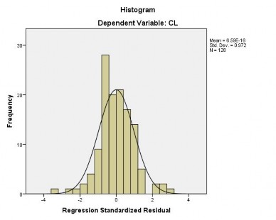
Figure 4.1: Histogram of residuals – normalized
(Source: Model testing results)
Regarding the PP Plot of standardized residuals, it can be seen that the observation points are not scattered far apart but concentrated near the expected diagonal, so the author concludes that the normal distribution of the residuals is not violated.
Figure 4.2: PP Plot of residuals – standardized
(Source: Model testing results)