continue to allocate a 1 , a 2 , a 4 into F 1 , allocate a 1 , a 2 , a 3 , a 4 into F 2 . The final result is F 1 = {a 1 , a 2 , a 4 , m 1 , m 4 , m 6 }, F 2 = {a 1 , a 2 , a 3 , a 4 , m 1 , m 2 , m 3 , m 5 }.
2.6.4. Algorithm evaluation
The fragmentation algorithm is correct because it satisfies three basic principles of fragmentation: Each attribute or method of a class is in one fragment; the class can be reconstructed from all its fragments because all fragments contain identifiers and identifier accessors; except for the identifier accessor, all other methods belong to only one fragment.
The complexity of the algorithm is determined by the following steps: If a class to be fragmented has a set of attributes A, a set of methods M, and a set of queries Q. The network consists of a set of stations S. The complexity of the algorithm
Maybe you are interested!
-

 Investment and Efficiency Estimates for Agricultural and Forestry Production Development Planning Scheme
 -
 Study on botanical characteristics, chemical composition and acetylcholinesterase enzyme inhibitory effects of two species Piper thomsonii (C. DC.) Hook. f. var. thomsonii and Piper hymenophyllum Miq., Piperaceae family - 24
 -
 Study on chemical composition, toxicity and some biological effects supporting the treatment of gastric and duodenal ulcers of Sanchezia nobilis Hook.F. leaves - 2
 -
 Study on botanical characteristics, chemical composition and acetylcholinesterase enzyme inhibitory effects of two species Piper thomsonii (C. DC.) Hook. f. var. thomsonii and Piper hymenophyllum Miq., Piperaceae family - 23
 -
 User Generated Database
2.1 and 2.2 are |C|*|Q|, the complexity of algorithm 2.3 is |C|*|M|*|Q|. The complexity of multiplying two matrices (step 3 in algorithm 2.6) is |M|*|Q|*|S|. The complexity of step 4 in algorithm 2.6 is |M|*|S|+|M|*|A|. So the complexity of algorithm 2.6 is (|C|*|Q|+|C|*|Q|+|C|*|M|*|Q|*|S|+|M|*|S|+|M|*|A|), this complexity is equivalent to (|C|*|M|*|Q|+|M|*|Q|*|S|).
Furthermore, the complexity of the N*N matrix multiplication algorithm has now been improved [36] to reach the complexity N 2.38 , so the complexity of step 3 in algorithm 2.6 is only N 2.38 with N being the largest of the three values |M|, |Q| and |S|.
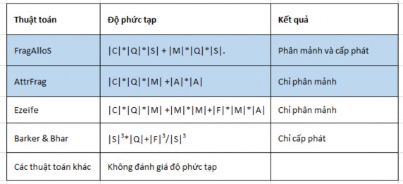
The key point of this algorithm is its ability to complete both the fragmentation and allocation phases with the above complexity while other algorithms that only perform one phase have equivalent complexity. For example, the complexity of Ezeife's vertical fragmentation algorithm [24] is |C|*|Q|*|M|
+|M|*|M|+|F|*|M|*|A|, the allocation algorithm of Barker and Bhar [13] has a complexity of |S| 3 *|Q|+|F| 3 /|S| 3 where |F| is the number of pieces (surely |F|>|C|).
The advantages of the heuristic approach in the FragAlloS algorithm can be listed as follows:
Among the methods, only the identifier access methods are repeated in all fragments.
Query and network information is used in both the fragmentation and allocation phases.
The complexity of the algorithm is low and depends on the number of classes, methods, queries and stations.
The maximum number of fragments is equal to the number of stations.
2.6.5. Experimenting with FragAlloS algorithm on OO7
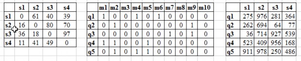
The algorithm randomly generates data sets including data matrix codes SSC, QMU, QSF. To demonstrate the effectiveness of the algorithm, the topic randomly selects the following data set:
Table 2.11: Table of experimental data with OO7
The fragmentation and allocation results to the stations after running the algorithm are as follows
- [m 1, m 3 , m 8 , m 10 ]->s 1
- [m 1 , m 6 ]->s 2
- [m 1 , m 7 , m 9 ]->s 3
- [m 1 , m 2 , m 4 , m 5 ]->s 4
Simulating test data with OO7 is done as follows:
- Use Module objects as stations
- The class to be evaluated will be extended from the existing OO7 AtomicPart object by adding methods as set in the above matrices.
With the above database schema design, the evaluation problem is performed according to 3 fragmentation options as follows:
- Option 1: The fragmentation and allocation option is generated according to the FragAlloS algorithm, shown in Figure 2.2.
- Option 2: Allocate all new methods to a station s 1 (or s 2 , s 3 , s 4 ), shown as Figure 2.3.
- Option 3: Random allocation, shown as Figure 2.4.
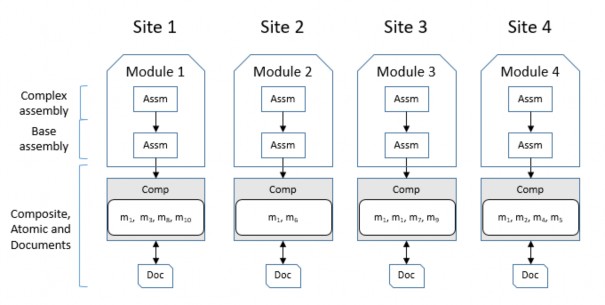
Figure 2.2: Fragmentation and allocation scheme generated by the FragAlloS algorithm
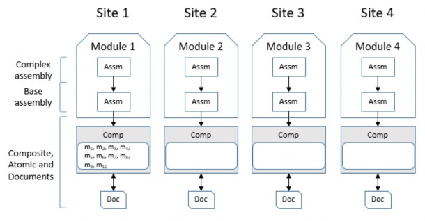
Figure 2.3: Non-fragmented and allocated plan at the same station s 1 (similar to s 2 /s 3 /s 4 )
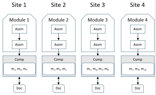
Figure 2.4: Fragmentation and random allocation scheme
The SSC matrix is implemented into the program by setting the cost as a fixed constant when there is a call from one station to another and this setting is fixed in all scenarios of running queries according to the QMU matrix. However, when executing queries q i (q 1 to q 5 ), the algorithm runs the same query q i in turn at stations s 1 to s 4 to produce different results for the same query q i .
The experimental results for each option have corresponding costs (calculated according to formula 2.1) in Tables 2.12, 2.13 and 2.14. The cost unit is determined by the unit of time multiplied by the unit of data size.
Table 2.12: Running results with option 1
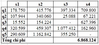
Table 2.13: Running results with option 2
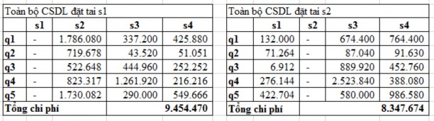
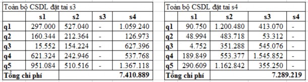
Table 2.14: Running results with option 3
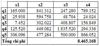
The costs of the options are represented in the chart in Figure 2.5. The experimental results show that the option generated by the FragAlloS algorithm (option 1) has the lowest cost.
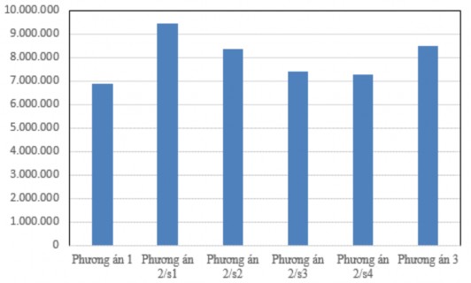
Figure 2.5: Chart comparing costs of options
2.7. Comparison of algorithms
Comparison of complexity: Table 2.15 is the result of the comparison of the complexity of the two proposed algorithms (FragAlloS and AttrFrag) with other algorithms. The FragAlloS algorithm has a complexity equivalent to Ezeife's algorithm, while Ezeife's algorithm only performs one phase, which is fragmentation.
Table 2.15: Comparison of algorithm complexity
Test setup:
The thesis has installed three algorithms FragAlloS, AttrFrag, Ezeife on Java language.
Experimental method: Because the two algorithms AttrFrag and Ezeife only perform fragmentation, the FragAlloS algorithm performs both fragmentation and allocation, the thesis proposes a cost calculation method (according to formula 2.1) to compare the three algorithms as follows:
o Get the fragmentation and allocation results of FragAlloS, calculate the cost, called FragAlloS _Cost
o Take the fragmentation result of AttrFrag, exhaustively check all allocation options to find the option with the smallest cost, called AttrFrag_minCost.
o Take the Ezeife fragmentation result, exhaustively check all allocation options to find the option with the smallest cost, called Ezeife_minCost.
Test data:
o Randomly generate QSF, QMU, MAU, SSC datasets
o Randomly generate data about the size of methods and properties.
Comparing the 3 costs FragAlloS _Cost, AttrFrag_minCost and Ezeife_minCost on the same datasets, the results are as follows:
o AttrFrag and Ezeife: 20% of the datasets give AttrFrag algorithm results with lower cost than Ezeife. 80% of the datasets give AttrFrag algorithm results with equal cost to Ezeife.
o FragAlloS and Ezeife: 70% of the datasets give results for FragAlloS algorithm with lower cost than Ezeife. 30% of the datasets give results for FragAlloS algorithm with equal cost to Ezeife.
The cost test results of the three algorithms on five datasets are shown in Table 2.16 and the cost comparison is shown by Figure 2.6.
Table 2.16: Costs of Ezeife, AttrFrag and FragAlloS algorithms
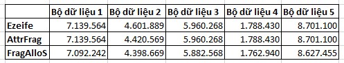
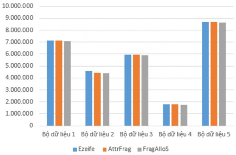
Figure 2.6: Cost comparison of Ezeife, AttrFrag and FragAlloS algorithms
2.8. Conclusion of Chapter 2
Fragmentation and allocation are logical database design techniques that reduce unnecessary accesses to data, allowing parallel execution of queries on fragments, thereby improving system performance. Because the object-oriented database model has its own characteristics such as encapsulation, inheritance, complex attributes and methods, to apply fragmentation methods from the relational model to the object model, it is necessary to transform the input parameters according to the class structure and relationships between classes in the object-oriented database.
The thesis proposes two fragmentation and allocation algorithms in the PT database:
(1) The AttrFrag algorithm fragments based on attribute correlation. (2) The FragAlloS heuristic algorithm performs fragmentation and allocation simultaneously with complexity