Evaluation of Classification Model Accuracy

- If not Begin

+ A  The attribute in the Attributes set has the best classification ability for the set

Examples

+ Decision attribute for Root node  A

+ For each value in the tree, 𝑣 𝑖 of attribute A

 Add a new branch under the Root node, corresponding to the case A = 𝑣 𝑖

 Determine the set 𝐸𝑥𝑎𝑚𝑝𝑙𝑒𝑠 𝑣 𝑖 as a subset of the set of Examples with value 𝑣 𝑖 of A

𝑖

 If 𝐸𝑥𝑎𝑚𝑝𝑙𝑒𝑠 𝑣 is empty

_ Under this new branch add a leaf node with the label being the most common value of the set

Target_attribute in the Examples set .

_ Else under this new branch add subtree

ID3 ( 𝐸𝑥𝑎𝑚𝑝𝑙𝑒𝑠 𝑣 𝑖 , Target_attribute, Attributes – {A} )

- End

- Return Root

By calculating the Gain value to select the optimal attribute for tree deployment, the ID3 algorithm is considered an improvement of the CLS algorithm.

When applying ID3 algorithm to the same input data set and trying multiple times, it gives the same result. Because, the candidate attributes selected at each step in the tree construction process are pre-selected.

However, this algorithm also does not solve the problem of continuous, numerical attributes, the number of attributes is still limited, and it has limited solutions to the problem of missing or noisy data.

2.1.5.3.3 C4.5 Algorithm

With

𝐺𝑎𝑖𝑛𝑅𝑎𝑡𝑖𝑜𝑛(𝑋, 𝑇) = 𝐺𝑎𝑖𝑛(𝑋,𝑇)

𝑆𝑝𝑙𝑖𝑡𝐼𝑛𝑓𝑜(𝑋,𝑇)

𝑆𝑝𝑙𝑖𝑡𝐼𝑛𝑓𝑜(𝑋, 𝑇) = − ∑ |𝑇 𝑖 | 𝑙𝑜𝑔

|𝑇𝑖|

(2.5)

(2.6)

𝑖∈ 𝑉𝑎𝑙𝑢𝑒(𝑋) |𝑇|

2 |𝑇|

In there:

- Value (X) is the set of values ​​of attribute X

- 𝑇 𝑖 is a subset of set T corresponding to attribute X = value is 𝑣 𝑖

For continuous attributes, we perform binary tests for all values ​​of that attribute. To efficiently collect the Entropy Gain value of all binary tests, we arrange the data according to the value of that continuous attribute using the Quicksort algorithm.

The C4.5 decision tree construction algorithm can be found in [21]. Some of the formulas used are

𝐼𝑛𝑓𝑜 (𝑇) = − ∑ 𝑛 |𝑇 𝑖 | ∗ 𝐼𝑛𝑓𝑜(𝑇 )

(2.7)

𝑥 𝑖=1 |𝑇| 𝑖

𝐺𝑎𝑖𝑛(𝑋) = 𝐼𝑛𝑓𝑜(𝑇) − 𝐼𝑛𝑓𝑜 𝑥 (𝑇) (2.8)

Formula (2.8) is used as the criterion for selecting attributes when classifying. The selected attribute is the attribute with the largest Gain value calculated according to (2.8).

Some improvements of C4.5 algorithm

- Working with multivalued attributes

The criterion (2.8) has a drawback that it does not accept multivalued attributes. Therefore, the C4.5 algorithm introduces the quantities GainRatio and SplitInfo ( SplitInformation ), which are determined by the following formulas:

𝑃 =

𝑓𝑟𝑒𝑞(𝐶 𝑗 , 𝑇)

|𝑆|

𝑆𝑙𝑖𝑝𝐼𝑛𝑓𝑜(𝑋) = − ∑ 𝑛

𝑇 𝑖

𝑇 𝑖

(2.9)

𝑖=1 𝑇 ∗ 𝑙𝑜𝑔 2 ( 𝑇 )

𝐺𝑎𝑖𝑛𝑅𝑎𝑡𝑖𝑜𝑛(𝑋, 𝑇) = 𝐺𝑎𝑖𝑛(𝑋,𝑇)

𝑆𝑝𝑙𝑖𝑡𝐼𝑛𝑓𝑜(𝑋,𝑇)

(2.10)

GainRatio is a criterion for evaluating the selection of classification attributes.

- Working with missing data

The algorithm just built is based on the assumption that all data samples have all the attributes. But in reality, there are missing data, that is, some data samples have attributes that are not defined, or are inconsistent or abnormal. Let us take a closer look at the case of missing data. The simplest way is not to include samples with missing values, otherwise it may lead to a lack of learning samples. Suppose T is a set of samples to be classified, X is a test according to attribute L, U is the number of missing values ​​of attribute L. Then we have:

𝐼𝑛𝑓𝑜(𝑇) = − ∑ 𝑘

𝑓𝑟𝑒𝑞(𝐶 𝑗 ,𝑇)

𝑓𝑟𝑒𝑞(𝐶 𝑗 ,𝑇)

𝑗=1

∗ 𝑙𝑜𝑔 (

2

|𝑇|− 𝑈

)

|𝑇|− 𝑈

(2.11)

𝐼𝑛𝑓𝑜

(𝑇) = − ∑ 𝑛

|𝑇|

∗ 𝑙𝑜𝑔 (𝑇 )

(2.12)

𝑥 𝑖=1 |𝑇|−𝑈

2 𝑖

In this case, when calculating the frequency freq ( 𝐶 𝑖 , 𝑇 ) we only calculate the samples with values ​​above the defined attribute L. Then the criterion (2.8) is rewritten using formula (2.13) as follows:

𝐺𝑎𝑖𝑛(𝑋) = |𝑇|

|𝑇|−𝑈

(𝐼𝑛𝑓𝑜(𝑇) − 𝐼𝑛𝑓𝑜 𝑥

(𝑇)) (2.13)

Similarly, change the criterion (2.13). If the test has N input values, then the criterion (2.13) is computed as if the original N sets were divided into (N+1) subsets.

Suppose the test X has values ​​𝑂 1 , 𝑂 2 … 𝑂 𝑛 selected in the standard way (2.13), how should we deal with missing data? Suppose the sample from the population T with output 𝑂 𝑖 is related to the population 𝑇 𝑖, then the probability that the sample belongs to the population 𝑇 𝑖 is 1.

Suppose each sample in 𝑇 𝑖 has an index that determines the probability of belonging to the set 𝑇 𝑖 . If the sample has attribute values ​​L, then it has a weight of 1. If in the opposite case, then this sample is related to the subset 𝑇 1 , 𝑇 2 … 𝑇 𝑛 with the corresponding probability:

|𝑇 1 |

|𝑇|−𝑈

|𝑇 |

2

,

|𝑇|−𝑈

|𝑇 |

𝑛

, … ,

|𝑇|−𝑈

(2.14)

We can easily see that the sum of these probabilities is equal to 1.

∑ 𝑛

|𝑇 1 | = 1

(2.15)

𝑖=1 |𝑇|−𝑈

In summary, this solution is stated as follows: The probability of missing values ​​occurring is directly proportional to the probability of non-missing values ​​occurring.

In this algorithm, the problem of working with numeric (continuous) attributes, attributes with multiple values ​​and the problem of missing and noisy data is solved. In C4.5, thresholding with numeric attributes is performed by binary separation, introducing the GainRatio quantity to replace the Gain quantity of ID3. To solve the problem of attributes with multiple values.

In addition, there is also an inappropriate pruning step. However, the weakness of this algorithm is that it does not work effectively with large databases because it does not solve the memory problem.

2.1.5.4 Pruning the decision tree

Through studying the decision tree construction algorithms above, we see that building a tree by growing the tree branches fully in depth to completely classify the training samples; such as the CLS algorithm and the ID3 algorithm sometimes have difficulty in cases where noisy data or missing data are not enough to represent a rule; that is, creating nodes with very small sample numbers. In this case, if the algorithm continues to grow the tree, it will lead to a situation that we call overfitting in the decision tree [2][3].

The overfitting problem is a difficulty in the study and application of decision trees. To solve this problem, people use the decision tree pruning method. There are two methods of pruning decision trees.

2.1.5.4.1 Prepruning

The pre-pruning strategy means that the tree will stop growing early before it reaches the point where the classification of the training examples is complete. That is, during the tree construction, a node may not be split further if the result of that split falls within a certain threshold. That node becomes a leaf node and is labeled with the label of the most common class of the set of examples at that node [2].

2.1.5.4.2 Postpruning

This strategy is the opposite of pre-pruning. It allows the tree to grow fully before pruning. That is, the tree is built first and then the branches that are not suitable are pruned. During the construction of the tree using post-pruning strategy, overfitting is allowed. If a node whose children are pruned, it becomes a leaf node and the leaf label is assigned the label of the most common class of its previous children [2][3].

In practice, post-pruning is a fairly successful method for finding highly accurate hypotheses. The post-pruning strategy is implemented by calculating the following errors:

Suppose we call: E(S) the static error (Static error or expected error) of a node S; BackUpError(S) the error from the child nodes of S (Back Up Error); Error(S) the error of node S. These values ​​are calculated as follows:

( 2.16)

𝐸 ( 𝑆 ) = (𝑁− 𝑛 + 1)

(𝑁+2)

In which: N is the total number of samples at node S, n is the number of samples of the most common class in S. In the general case, if the class attribute has K values ​​(K classes then:

𝐸 ( 𝑆 ) = (𝑁− 𝑛 + 𝐾− 1)

(𝑁+𝐾)

In which: 𝑆 𝑖 is a child node of S, 𝑃 𝑖 is the ratio of the number of samples in 𝑆 𝑖 to the number of samples in S.

Thus, the leaf nodes will have an error Error ( 𝑆 𝑖 ) = E ( 𝑆 𝑖 ) because the leaf node has no children, leading to no BackUpError. If BackUpError (S) ≥ E (S), then the post-pruning strategy decides to cut at node S (i.e., remove the children of S).

In summary, tree pruning aims to: optimize the resulting tree. Optimize the tree size and the accuracy of the classification by removing inappropriate branches (over fitted branches). To perform tree pruning, there are the following basic techniques [1] [2] [3].

- Use the disjoint set of training samples to evaluate the usefulness of post-pruning nodes in the tree. Using this tree pruning technique is the CART algorithm, abbreviated as cost complexity.

- Apply statistical methods to evaluate and prune branches with low reliability or further extend branches with high accuracy. This pruning technique is called pessimistic pruning and is often used to prune trees built by ID3 and C4.5 algorithms.

- Minimum length description technique. This technique does not require checking the patterns and it is commonly used in SLIQ, SPRINT algorithms.

2.1.5.5 Evaluation of the accuracy of the classification model

Estimating the classifier's accuracy is important because it allows us to predict the accuracy of future classification results. Accuracy also helps to compare different classification models. There are two popular evaluation methods: Holdout and k-fold cross-validation . Both techniques rely on random partitioning of the initial data set.

2.1.5.5.1 Holdout Method

The output data is randomly divided into two parts: training data set and testing data set. Usually 2/3 of the data is given to the training data set, the remaining part is given to the testing data set [2].

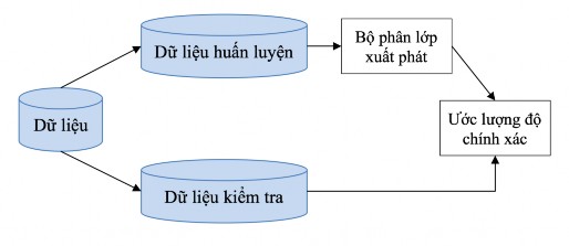
Figure 2-6: Holdout Method

2.1.5.5.2 K-fold cross-validation method

Cross-validation is a statistical method of evaluating and comparing learning algorithms by dividing the data into two segments: one segment used to train a model and another segment used to validate that model.

Cross-validation is used to estimate the performance of a model learned from available data using an algorithm. In other words, to evaluate an algorithm in general. Cross-validation is also used to compare the performance of two or more different algorithms and determine the best algorithm for the available data, or alternatively to compare the performance of two or more variants of a parametric model [3].

k-fold cross-validation method: The initial data set is randomly divided into k subsets (folds) of approximately equal size S 1 , S 2 …, S k . The learning and testing process is performed k times. At the i-th iteration, S i is the testing data set, the remaining sets form the training data set. That is, training is first performed on the sets S 2 , S 3 …, S k , then testing on

set S 1 ; the training process is continued on the sets S 1 , S 2 , S 4 ,…, S k , then tested

on set S 2 ; and so on for the remaining sets.

Accuracy is the total number of correct classifications from k iterations divided by the total number of samples in the original dataset [27][23].

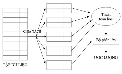
Figure 2-7: K-Fold Coss–Validation