Dva Distance Vector Routing Algorithm

The non-negative weights of the edges of a graph are more general than the geometric distances between their endpoints. For example, given three vertices A, B, C, the path ABC may be shorter than the direct path AC.

3.4.4.1.2. Algorithm

Dijkstra's algorithm can be described as follows:

Maybe you are interested!

We manage a dynamic set S . Initially S={s} .

For each vertex v, we maintain a label d[v] that is the minimum length of the paths from source s to some vertex u in S , and then follow the edge connecting uv.

Among the vertices outside S , we choose the vertex u with the smallest label d[u] and add it to the set S. The set S is expanded by one more vertex, then we need to update the labels d to match the definition.

The algorithm ends when all vertices are in the set S, or if we only need to find the shortest path to a destination vertex t, then we stop when vertex t is added to the set S.

The non-negativity of edge weights is closely related to the correctness of the algorithm. We must use this property when proving the correctness of the algorithm.

3.4.4.1.3. Proof

The idea is demonstrated as follows:

We will show that, when a vertex v is added to the set S, then d[v] is the value of the shortest path from source s to v.

By the definition of label d, d[v] is the value of the shortest path among the paths from source s, through vertices in S, and then along an edge directly connecting uv to v.

Suppose there exists a path from s to v with a value less than d[v] . Thus, in the path, there exists a vertex between s and v that does not belong to S. Choose w as the first such vertex.

Our path is of the form s - ... - w - ... - v. But since the weights of the edges are non-negative, the length of the segment s - ... - w is no greater than the length of the entire path, and therefore has a value smaller than d[v] . On the other hand, because of our choice of w, the length of the segment s - ... - w is d[w] . Thus d[w] < d[v] , which is contrary to the choice of vertex v. This is a contradiction. So our assumption is wrong. We have something to prove.

3.4.4.1.4. Implementation steps

The Dijkstra algorithm used in the 0SPF routing protocol goes through the following steps:

1. The router constructs the network graph and identifies the source and destination nodes, say V 1 and V 2 . It then constructs a matrix, called the adjacency matrix. This matrix represents the weights of the edges, say [i,j] is the weight of the edge connecting V i to V j . If there is no direct connection between V i and V j , this weight is defined to be infinity.

2. The router builds a state table for all nodes in the network. This table consists of the following parts:

 Length: represents the magnitude of the weight from the source to that node.

 Node label: represents the state of the node, each node can have one of two states: fixed or temporary.

3. The router assigns initial state table parameters to all nodes and sets their length to infinity and their labels to temporary.

4. The router sets up a T-node. For example, if V 1 is the source T-node, the router will change the label of V 1 to permanent. Once a label changes to permanent, it will not change again.

5. The router will update the state table of all temporary nodes that are associated with the source T-node.

6. The router looks at the temporary nodes and chooses a single node whose weight to V 1 is the smallest. This node then becomes the destination T-node.

7. If this node is not V 2 then the router returns to step 5.

8. If this node is V 2 then the router removes its previous node from the state table and keeps doing this until it reaches node V 1 . The nodes in turn determine the optimal route from V 1 to V 2 .

3.4.4.1.5. Example of Dijkstra's algorithm

Below we will find the shortest path between A and E.

Step 1 : According to the following figure, node A is the source node T-node, its label is changed to fixed and marked with

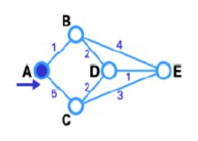
Step 2 : In this step, we will see the state table of the nodes directly connected to node A, which is the pair of nodes (B,C). The path from A to B is the shortest (has the smallest weight), so it is chosen as T-node and then its label is changed to fixed.

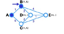
Step 3 : same as step 2, based on the state table of the nodes directly connected to node B is the pair of nodes (D,E). Similarly, node D connected to node B is the shortest path (with weight 2 so it is smaller than the weight of edge BE), so node D is made T-node, and then its label is changed to fixed.

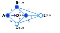
Step 4 : In this step we don't have any temporary node, so we can only select the next T-node. Node E is selected in the graph, edge DE has the smallest weight.

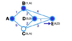
Step 5 : Node E is the destination node so we end this routing process.

3.4.4.2. DVA Distance Vector Routing Algorithm

It is a routing algorithm that calculates the shortest path between pairs of nodes in a network, known as the Bellman-Ford algorithm. Network nodes exchange information on the basis of the destination address, the next node, and the shortest path to the destination. Each node in the network has a routing table that shows the best path to every destination, and each node sends its routing table only to its neighbors.

The problem with the DV algorithm is that it counts to infinity when a connection is broken. This problem can be seen clearly in the following example:

Figure 3.7: Example of DVA algorithm

Figure 3.7 shows that there is only one route between node A and other nodes. Suppose the weight on each edge is equal to 1, each node (Router) has a routing table. Now, if we cut the connection between A and B, node B will revise its routing table. After some time, the nodes exchange routing table information and B receives C's routing table. Since C does not know what happened to the connection between A and B, it will assume that there is a route with weight 2 (1 for connection CB and 1 for connection BA), it does not know that connection AB has been cut. B receives this routing table and thinks that there is another route between C and A, so it revises its routing table and changes the weight of connection BA to 3 (1 for connection BC, 2 for connection CA). Again the nodes change their routing table. When C receives B's routing table, it sees that B's table changes the weight of route BA from 1 to 3, so it updates its routing table and changes the weight of route CA to 4 (1 for the CB connection and 3 for the BA connection). This process continues until all nodes find that the weight of the route to A is infinite.

The Bellman-Ford algorithm is an algorithm for computing the shortest paths in a weighted directed graph (in which some edges may have negative weights). The Dijksta algorithm requires the weights of the edges to be non-negative. Therefore, the Bellman-Ford algorithm is often used when there are edges with negative weights.

3.4.4.2.1. Algorithm

The Bellman-Ford algorithm can be stated as: Find the shortest paths from a given source node with the constraint of containing only one route, then find the shortest path with the constraint of containing only two routes at most, and so on. If the previous path is the shortest, leave it, otherwise update the new path. The algorithm proceeds through the layers shown below:

function BellmanFord (vertex_list, arc_list, source)

// function requires input graph as a vertex list, an arc list

// function to calculate distance and previous_vertex values of vertices, so that

//previous_vertex_value will save the shortest paths.

// step 1: initialize graph

for each v in vertex_list:

if v is source then distance (v) := 0 else distance (v) := infinity previous_vertex (v) := null

// step 2: edge admission

for i from 1 to size (vertex_list) :

for each (u, v) in list_of_arcs:

if distance (v) > distance (u) + weight (u, v) : distance (v) := distance (u) + weight (u, v) previous_vertex (v) := u

// step 3: check negative cycle

for each (u, v) in list_of_arcs:

if distance (v) > distance (u) + weight (u, v) :

error “Graph contains negative weighted cycle”

3.4.4.2.2.Proof

The correctness of an algorithm can be proven by induction. The algorithm can be stated precisely inductively as follows:

Theorem: After i iterations of the for loop:

1. If Distance(u) is not infinitely large, then it is equal to the length of some path from s to u;

2. If there is a path from s to u through at most i edges, then Distance(u) has a value not exceeding the length of the shortest path from s to u through at most i edges.

Prove:

Base case: Consider i = 0 and the time before the for loop is run for the first time. Then, for the source vertex distance(source) := 0, this is true. For other vertices u, distance(u) := infinity, this is also true because there is no path from source to u through 0 edges.

Inductive case:

Proof of statement 1: Consider the moment when the distance to a vertex is updated by the formula distance (v) := distance (u) + weight (u,v). By the inductive assumption, distance (u) is the length of a path from the source to u. Therefore, distance (u) + weight (u, v) is the length of the path from the source to u and then to v.

Proof of statement 2: Consider the shortest path from the source to u through at most i arcs. Suppose v is the vertex immediately before u on this path. Then, the path from the source to v is the shortest path from the source to v through at most i-1 arcs. According to the inductive hypothesis, the distance (v) after i-1 iterations does not exceed the length of this path. Therefore, the weight (v, u) + distance (v) has a value that does not exceed the length of the path from s to u. In the i-th iteration, the distance (u) is taken as the smallest value of the distance

(v) + weight (v, u) for all possible v. Therefore, after i iterations, the distance (u) has a value that does not exceed the length of the shortest path from the source to u through at most i edges. When i is equal to the number of vertices in the graph, each path found will be a global shortest path, unless the graph has a negative cycle. If there exists a negative cycle that can be reached from the source vertex, then there will be no shortest path (because each time around the negative cycle is a decrease in the path's weight).

3.4.5. Conclusion

Both algorithms work under static conditions of network topology and path cost, then both converge to a solution. When the network has many changes, the algorithm will try to follow the changes, however, if the path cost depends on the traffic, that is, it depends on the chosen path, then the response makes the network unstable.

3.5. WAVELENGTH ASSIGNMENT

Wavelength assignment is a major factor affecting the probability of congestion and the performance of the network. Appropriate wavelength assignment can reduce the number of wavelengths used or eliminate the need for wavelength converters, thus greatly reducing the cost of the network. Wavelength assignment is divided into two types for fixed network traffic and variable network traffic. When the network traffic is fixed, the assignment is fixed, the same wavelength is assigned if (if available) to every request made at a node, otherwise the request is blocked. When the network traffic is variable, when a request arrives at a certain network node, that node will use an algorithm to select a particular wavelength that is free at that node and assign it to that lightpath to route it, otherwise the request is blocked.

The request is not resolved. The algorithm for the assignment method maintains a list of used wavelengths and free wavelengths at each node.

Wavelength assignment methods are divided into the following types:

 Random assignment type : when a request comes to a node, that node will determine the steps

The wave is still valid (i.e. still idle) and randomly selects one

 i in wavelengths

to assign to that request. The available wavelengths at each node are determined by

wavelength elimination

 i has been removed from the list of free wavelengths; when the call ends

push,

 i is removed from the busy wavelength list and added back to the list

initially free wavelengths. This method does not require information about the entire network state when performing wavelength assignment. This assignment distributes traffic arbitrarily, so wavelength utilization is balanced and wavelength contention is low, so the probability of congestion is also lower.

 First-Fit assignment : this assignment will find and assign wavelengths in a fixed order. All wavelengths are numbered from low to high and the wavelengths selected for assignment are also indexed from low to high, that is, the first wavelength selected is the wavelength with the smallest index among the free wavelengths and assigned to the request. Similar to the Random assignment method, this assignment does not require any information about network status information. The limitation of this method is that wavelengths with smaller indexes are used more, while wavelengths with larger indexes are hardly used. Furthermore, increasing the number of wavelengths in the fiber does not bring any effect because wavelengths with higher indexes are rarely used. Therefore, the contention for wavelengths with smaller indexes increases, which also increases the probability of congestion. This assignment gives lower cost than Random assignment because it does not need to check all wavelengths in each path, so it is preferred.

 Least-used assignment : This assignment selects the wavelengths that are least used in the network. The purpose of this assignment is to balance the load across all wavelengths. This assignment requires network state information to find the least-used wavelength. However, this method is expensive in terms of storage and computation costs.

 Most - used assignment : it is the opposite of Least-used assignment, it finds the most used wavelengths in the network. This assignment requires information about the network state to find the most used wavelengths.

It also incurs the same costs as in Least-used assignment, however it performs better than Least-used assignment.

For the above wavelength assignments, Random and First-Fit are more practical because they are easy to implement. Unlike Least-used and Most-used methods which require network information. It simply relies on the current node state and selects a wavelength from the available wavelengths at that output connection. Relatively, Random method gives better performance than First-Fit method.

To implement the Least-used and Most-used assignment methods, each node needs to be equipped with the entire network information. So these methods depend on the intelligence and accurate understanding of the nodes. Since the network state changes rapidly, it is difficult to know the exact network information at all times, thus affecting the wavelength assignment. Moreover, nodes exchange information with each other about the network at fixed intervals and this information will consume a significant amount of bandwidth, thus reducing the bandwidth available for data transmission.

3.6. VIRTUAL PATH ESTABLISHMENT

A virtual path is considered a path of light from source to destination. When a call request is made at a node, the node uses a routing and wavelength assignment algorithm to find a path and a wavelength for that call. The node assigns the chosen wavelength to the call and routes it to the next node. At each intermediate node along the path, the wavelength of the incoming lightpath is checked to see if it is available to be assigned and from there to continue. If that wavelength is not available, and if the node has a wavelength converter, it can switch to another wavelength to route the lightpath. The newly established path is called a virtual path, and is established before any data is transmitted.

A physical path consists of all the transmission links formed on the path from source to destination, but the virtual path may contain the same or different wavelengths from source to destination. Two requests for calls with the same source and destination endpoints may have the same physical path but different virtual paths. The following figure shows the formation of a lightpath. Here two calls are initiated from node 1 and the virtual path for each call is drawn. For the first call, node 1 assigns the wavelength

 1 and send it to node 2. Suppose node 2 has a wavelength converter but no

available wavelength

 1 , so it shifts to wavelength

 2 and send to node 3. Node 3 assigns next

Comment