Step 3. Continue repeating step 2 to add precedent levels (if any).
 Find cell dependencies
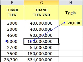
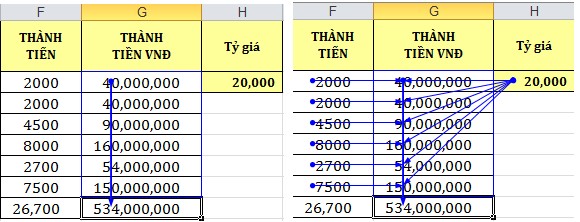
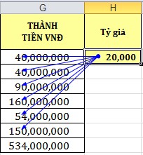
Step 1. Select the cell containing the formula whose Dependent you want to find.
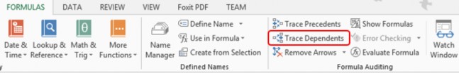
Step 2. Select Tab Formulas Group Formula Auditing Trace Dependents
Step 3. Continue repeating step 2 to add Dependent levels (if any).
 Remove Tracer Arrows
Select Formulas Tab Group Formula Auditing Remove Arrow s
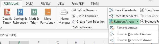
To remove precedent arrows one level at a time, select Remove Precedent Arrows.
To remove dependent arrows one level at a time, select Remove Dependent Arrows.
 Common error messages
When Excel fails to calculate a formula, the program will report an error message, starting with the # sign . Below is a list of common error messages.
Error message
Reason | |
#DIV/0! | The formula contains division by 0. |
#N/A | The formula refers to a cell with a value that cannot be found, or the function entry is missing an argument. |
#NAME? | The formula contains an incorrect function name or cell name. |
#NULL | Occurs when an intersection of two regions is determined but the intersection region is empty. |
#NUM! | The numerical data is incorrect. |
#REF! | Occurs when a formula contains a reference to an invalid address. |
#VALUE! | The formula contains operands and operators of the wrong type. |
Maybe you are interested!
-
 Advanced XML Web Programming - Dalat College of Technology - 10
 -
 Advanced XML Web Programming - Dalat College of Technology - 1
 -
 Advanced XML Web Programming - Dalat College of Technology - 5
 -
 Designing teaching activities for the lesson Parallel force rule. Equilibrium conditions of solids under the action of three parallel forces and the lesson Caucasus's law. Absolute temperature Advanced Physics 10 textbook to promote students' initiative and autonomy in learning - 9
 -
 Organizing project-based learning in advanced mathematics for engineering university students - 13
 Fix formula errors
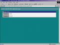
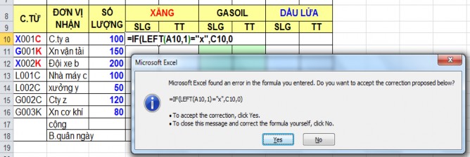
If you miss a parenthesis when entering a formula, or if you put a parenthesis in the wrong place, Excel often displays a dialog box like the one shown below when you try to confirm the formula. If the formula (suggested by Excel in the dialog box) is what you want, click Yes to have Excel automatically correct the formula for you; if the formula is incorrect, click No and correct the formula yourself.
 Use the formula error checking function
If you use Microsoft Word, you're probably familiar with the blue wavy lines that appear under words or phrases that the grammar checker thinks are incorrect. Grammar checkers work by using a set of rules to check grammar and syntax. As you type, the grammar checker silently monitors your every word, and if something you type doesn't follow the grammar checker's rules, a wavy line appears to let you know there's a problem.
Excel has a similar feature: the formula error checker. It’s similar to a grammar checker, using a set of rules to check calculations, and it also works silently while monitoring your formulas. If it detects something wrong, it displays an error indicator—a green triangle—in the upper left corner of the cell containing the formula.
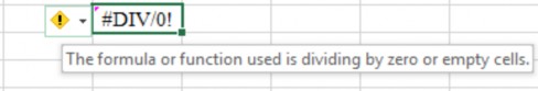
How to fix the error
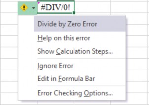
When you select a cell with an error, Excel displays a smart tag next to it, and if you hover over the newly created icon, a message describing the error will appear, as shown in the image above. There is also a button on the right side of the icon that opens a list of possible solutions to the error:
- Help on This Error: Find information about errors through Excel's Help system.
- Show Calculation Steps : Run the Evaluate Formula function.
- Ignore Error: Ignore, keep the wrong formula as it is.
- Edit in Formula : Displays the formula in edit mode on the formula bar. It is simply to let you edit the formula yourself.
- Error-Checking : Shows the options of the Error Checking function from the Option dialog box for you to choose.
Set options for error checking
Just like the grammar checker in Word, the Formula Error Checker has a number of options to determine how it works and what errors it will flag. To see these options, you have two ways:
- Select Office, Excel Options to display the Excel Options dialog box, and select Formulas
- Select Error-Checking Options in the drop-down list of the error icon (as mentioned in the previous post).
Both methods open up options for Error Checking and Error Checking Rules as illustrated:
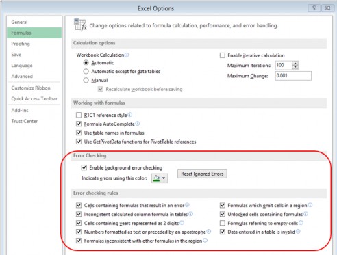
Enable Background Error Checking : This check box turns the automatic mode of the Formula Error Checker function on and off. If you turn this mode off, every time you want to check for formula errors, you choose Formulas, Error Checking.
Indicate Errors Using This Color : Choose a color for the error indicator (the tiny triangle in the left corner of the cell with an error).
Reset Ignored Errors : If you have ignored one or more errors, you can display them again by pressing this button.
Cells Containing Formulas That Result in an Error : When this option is enabled, the Formula Error Checker will highlight formula cells that result in error values such as #DIV/0!, #NAME?, or any previously used error values.
Inconsistent Calculated Column Formula in Tables : (New option in Excel 2007) When this option is enabled, Excel checks the
formulas in a calculated column of a Table (a special type of Excel table), and highlights cells with formulas whose structure is different from other formulas in the column. The smart tag in the cell with the error includes a Restore to Calculated Column Formula command, which allows you to update the formula so that it is consistent with the formulas in the rest of the column.
Cells Containing Years Represented as 2 Digits : When this option is enabled, the Formula Error Checker flags formulas that include dates in which the year number has only 2 digits (an ambiguous situation, because the string could refer to a date in either 1900 or 2000). In this case, the list of options in the smart tag contains two commands — Convert XX to 19XX and Convert XX to 20XX — that let you convert a 2-digit year number to a 4-digit number.
Numbers Formatted as Text or Preceded by an Apostrophe : When this option is enabled, the Formula Error Checker will highlight cells that contain a number formatted as text or preceded by an apostrophe ('). In this case, the list of options in the smart tag includes a Convert to Number command to convert the number into an actual number (formatted as a number).
Formulas Inconsistent with Other Formulas in the Region : When this option is enabled, the Formula Error Checker will flag formulas that are structured differently from similar formulas around them. In this case, the list of options in the smart tag includes a command like Copy Formula from Left to make this formula consistent with the surrounding formulas.
Formulas Which Omit Cells in a Region : When this option is enabled, the Formula Error Checker will highlight formulas that omit rows adjacent to the range referenced in the formula.
Unlocked Cells Containing Formulas : When this option is enabled, the Formula Error Checker will mark formulas in cells that are unlocked. This is not an error but a warning that others can modify the formula, even after you have protected the worksheet. In this case, the list of options in the smart tag includes the Lock Cell command, which locks the cell and prevents other users from changing the formula after you have protected the worksheet.
Formulas Referring to Empty Cells : When this option is enabled, the Formula Error Checker will flag formulas that refer to empty cells. In this case, the list of options in the smart tag includes a Trace Empty Cell command that allows you to find the empty cell that the formula is referring to (and you can enter data into that empty cell, or adjust the formula so that it no longer refers to this cell).
Data Entered in a Table Is Invalid : When this option is enabled, the Formula Error Checker will highlight cells that violate the data-validation rules of a table. This can happen if you set a Data-validation rule with only a Warning or Information type, users can still choose to enter invalid data in this case, and the Formula Error Checker will highlight cells containing invalid data. The options list in the smart tag includes a Display Type Information command, which displays the Data-validation rule that the cells violate.
 Using Watch Window
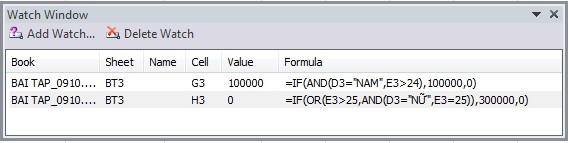
This feature helps us monitor cells during the calculation process. If you want to monitor a cell, add it to the monitoring list in the Watch Window . Call the Watch Window :
- Select Formulas Tab Formula Auditing group Watch Window
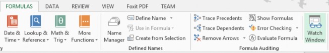
Figure 2.2.12
- Then select the cell to monitor and click the Add Watch button on the window.
Watch Window .
 Using Data Validation function in data entry management
When building any spreadsheet for your work, you will definitely need certain required data entry areas. That data can be
is limited to a certain range, which can be integers, decimals, dates, times, in an available list or strings of a certain length. Then the Data validation function will help us enter data accurately as required, minimizing errors.
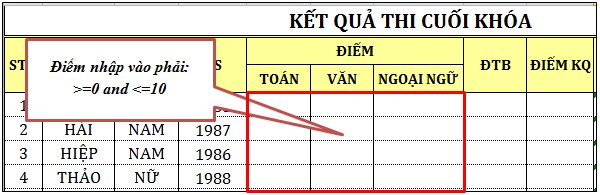
Example: Input score must be >=0 and <=10:
To set up conditional input, do the following:
Step 1. Select the area you want to set conditions for.
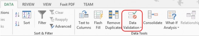
Step 2. Go to Data Tab group Data Tools Data Validation
Figure 2.2.15
Step 3. In the Data Validation dialog box as shown below, there are three Tabs Settings, Input Message, Error Alert.
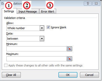
1. Settings tab