Resource Restructuring Methodology

of M-PSO is 85.3. From this result, it can be seen that the M-PSO algorithm is more efficient than the GA-M algorithm and the stability of M-PSO is also better.

Comparison with other hybrid algorithms

- Table 2.13 shows that the results of M-PSO are better than hybrid algorithms in most cases, specifically: better than HAntCO 29/30 data sets, better than GRASP 27/30 data sets with BEST value, 26/30 data sets with AVG value. Some cases M-PSO is worse than hybrid algorithms, however, the worse value is not much. For example, when compared with GRASP algorithm, the worst case of M-PSO compared to GRASP is -7.04%, while the best value is higher than GRASP is 15.79%.

Thus, in the new algorithm M-PSO with the addition of the population migration method, it has brought good efficiency to the algorithm. The nature of population migration is to expand the search space, helping the algorithm to be able to scan and browse more solutions, thus being able to find better solutions. In addition, the migration method helps the new algorithm to easily escape local extrema.

2.3.5. Comparison image of M-PSO and GA-M

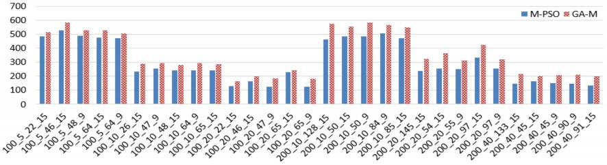
Figure 2.5. Comparison of BEST values between M-PSO and GA-M

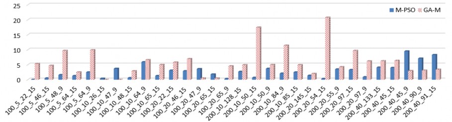
Figure 2.6. Comparison of STD values between M-PSO and GA-M

2.4. Proposed DEM algorithm

The DEM (Reallocate Differential Evolution for MS-RCPSP) algorithm [CT7], [CT8] is built on the basis of the DE algorithm to solve the MS-RCPSP problem. The goal of this algorithm is to find the schedule with the shortest execution time. DEM is applied to MS-RCPSP with the following improvements:

For the best individual after each generation, apply the method of finding and replacing the resources that perform the tasks of the individual. This method is called resource re-establishment.

2.4.1. Method of re-establishing the implementation resources

2.4.1.1. Idea of the reconstruction method

In the MS-RCPSP problem, a schedule is an individual representing the resources that perform the task that satisfies the initial constraints. After each generation, the algorithm will find the best schedule (C best ), based on this schedule, continue to change the resources that perform each task so that the constraints of the problem are still met. Changing the resources that perform the task is called the Reallocate method. This method helps to expand the search space and can avoid local extrema.

The reset method is performed through the following steps:

- Step 1: Find the most used resource in C best , called L b . This is the resource that finishes work last among the resources used to carry out the project.

- Step 2: Browse each task performed by resource L b in turn according to the execution priority of the tasks on the schedule.

W R b : set of tasks being performed by L b

- Step 3: For each task W i ∈ W R b (i=1- sizeof(W R b )) , do:

• Find all resources that are capable of performing task W i other than the current resource ( L b ) , denoted by L W ;

• Iterate through each resource that can perform task Wi , for each resource L j W ∈ L W , do:

o (1) Set the execution resource W i as R j W ;

o (2) Remove W i from the task list that L b is performing.

After (1) and (2) we will get the new schedule, calculate the makespan of the new schedule new best , if it is better than the makespan of C best , replace C best with the new best schedule and stop, otherwise, continue to execute the loop to check.

𝐶𝑏𝑒𝑠𝑡

{ 𝑛𝑒𝑤 𝑏𝑒𝑠𝑡 𝑖𝑓 𝑓(𝑛𝑒𝑤 𝑏𝑒𝑠𝑡 ) < 𝑓(𝐶 𝑏𝑒𝑠𝑡 )

𝐶 𝑏𝑒𝑠𝑡 𝑖𝑓 𝑓(𝑛𝑒𝑤 𝑏𝑒𝑠𝑡 ) ≥ 𝑓(𝐶 𝑏𝑒𝑠𝑡 )

This shift helps the algorithm expand the search space by generating new individuals based on the best individual. Since the new best individual is generated from the best individual, it is possible to use the experience of both the population and the best individual over generations, which is the characteristic of the DE algorithm. Therefore, after applying Reallocate, we can get better individuals.

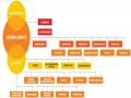
2.4.1.2. Algorithm diagram

The implementation steps of the reconstruction method are shown in detail in the algorithm diagram in Figure 2.7.

2.4.1.3. Reallocate function

The resource re-establishment algorithm [CT7], [CT8] performs the task detailed in Algorithm 2.2 below.

Algorithm 2.2. Reallocate

Input: currentBest (best instances after each generation)

Output: schedule after correction

Maybe you are interested!

1. makespan = f(currentBest)

2. newbest = currentBest;

3. L b = lastResource (newbest) // last completed resource

4. W b = {tasks performed by L b }

5. For i=1 to size(W b ) // iterate over each task in turn

6. W i = W b [i]; // get the i- th task

7. Li = {resources to be executed W i # L b }

8. For j = 1 to size(L i ) // iterate over each resource in turn

9. L i [j] = L i [j] + {W i } // convert ti to L i [j]

10. L b = L b – {W i } // remove Wi from L b

11. newmakespan = f(newbest) // recalculate makespan

12. If newmakespan < makespan

13. makespan = newmakespan

14. Return newbest; // successful move, return result and stop function

15. End if

16. newbest = currentBest; // shift fails, get back the original schedule (before shift) to execute the next loop

17. End for // j

18. End for // i

19. Return newbest;

End Function

With:

- f: function to calculate the makespan of a schedule

- size: function to calculate the number of elements in a set/array

- lastResource: function returns the last resource to finish executing

Example 2.3:

Consider a project with the following information:

- Task set W ={1, 2, 3, 4, 5, 6, 7, 8, 9, 10}

- Resource set L = {1, 2, 3}.

Begin

new best = C best ; makespan = f(new best )

W R

L b = max(new best ); i=0

b = {tasks in L b }

i++; i < size(W R )

Wrong

Correct

W i ∈ W R , i=1.. size( W R ); j=0

L t = {realizable resource set Wi } # L b

j++; j < size(L t )

Add Wi to L t j Remove Wi from L b

f(new best ) < makespan

Wrong

Correct

C best = new best makespan = f(new best )

End

Figure 2.7. Block diagram of task migration to another resource

The task execution time is shown in table 2.14.

Table 2.14: Time to perform tasks

Task

1	2	3	4	5	6	7	8	9	10
Time	2	4	3	5	2	2	5	3	4	2

Figure 2.8 shows the relationship between tasks. Specifically as follows:

- Task 2 is done and completed before tasks 6 and 8 start;

- Task 3 is done and completed before task 7 starts;

- Task 4 is done and completed before task 5 begins;

- Task 8 is done and completed before task 9 starts;

- Task 5 is done and completed before task 10 begins.

Task 0 and task 11 are two dummy tasks with a duration of 0, representing the start and end times of the project.

W 6

W 2

W 8

W 9

W 0

W 1

W 3

W 7

W 11

W 4

W 10

W 5

Figure 2.8. Priority order of tasks The capacities of the resources are given in Table 2.15.

Table 2.15: Resource capacities

Task

W 1	W 2	W 3	W 4	W 5	W 6	W 7	W 8	W 9	W 10
L 1	×	×	×	×			×		×	×
L 2	×		×	×	×	×		×	×
L 3	×		×		×		×	×		×

Suppose, after one generation, we find a schedule with task resources set up as in table 2.16.

Table 2.16: Task execution resources

Task

1	2	3	4	5	6	7	8	9	10
Resources	1	1	2	1	2	2	3	2	1	1

We can see, the Gantt chart of schedule 2.15 is as shown in figure 2.9 below. The Makespan of schedule 2.15 is: 17

L 1

W 1		W 2				W 4					W 9				W 10
L 2			W 3			W 5		W 6		W 8
L 3						W 7
Time	1	2	3	4	5	6	7	8	9	10	11	12	13	14	15	16	17

Figure 2.9. Gantt chart of schedule 2.15

Applying the Reallocate function, we set the resource to perform task W 9 as L 2 , the new schedule is shown in Figure 2.10. The new schedule has a makespan of 16, which is better than the previous result.