

Table 2.2 Stationarity test results of base money factors
Variable
Level | Delay | Value of KĐ | ADF Critical Value Stationarity 1% 5% 10% | |
Q | Q | 1 | -0.3945 | -3.6353 -2.9499 -2.6133 No stop |
D(1) | 1 | -4.8370 | -3.6422 -2.9527 -2.6148 1% Line | |
C/DD | C/DD | 1 | -3.3626 | -3.6353 -2.9499 -2.6133 5% range |
D(1) | 1 | -4.6686 | -3.6422 -2.9527 -2.6148 1% Line | |
Dr | Dr | 1 | -2.2217 | -3.6353 -2.9499 -2.6133 No stop |
D(1) | 1 | -3.2071 | -3.6422 -2.9527 -2.6148 5% range | |
YAG/Y | YAG/Y | 1 | -4.1330 | -3.6353 -2.9499 -2.6133 1% Line |
D(1) | 1 | 5.7582 | -3.6422 -2.9527 -2.6148 1% Line | |
TD | TD | 1 | -1.3198 | -3.6353 -2.9499 -2.6133 No stop |
D(1) | 1 | -6.9706 | -3.6422 -2.9527 -2.6148 1% Line | |
YNA/Y | YNA/Y | 1 | -4.1330 | -3.6353 -2.9499 -2.6133 1% Line |
D(1) | 1 | -5.7582 | -3.6422 -2.9527 -2.6148 1% Line | |
TD/DD | TD/DD | 1 | -0.8524 | -3.6353 -2.9499 -2.6133 No stop |
D(1) | 1 | -5.7976 | -3.6422 -2.9527 -2.6148 1% Line | |
Lr | Lr | 1 | -3.5976 | -3.6353 -2.9499 -2.6133 5% range |
D(1) | 1 | -4.5453 | -3.6422 -2.9527 -2.6148 1% Line | |
Er/D | Er/D | 1 | -2.0491 | -3.6353 -2.9499 -2.6133 No stop |
D(1) | 1 | -4.7461 | -3.6422 -2.9527 -2.6148 1% Line | |
Br | Br | 1 | -0.8928 | -3.6353 -2.9499 -2.6133 No stop |
D(1) | 1 | -4.3274 | -3.6422 -2.9527 -2.6148 1% Line | |
Rr | Rr | 1 | -2.3791 | -3.6353 -2.9499 -2.6133 No stop |
D(1) | 1 | -4.3015 | -3.6422 -2.9527 -2.6148 1% Line | |
LA/TL GDP | LA/TL | 1 | -1.1438 | -3.6353 -2.9499 -2.6133 No stop |
D(1) | 1 | 3.8837 | -3.6422 -2.9527 -2.6148 1% Line | |
GDP | 1 | 2,525 | -2.6162 -1.9481 -1.612 5% Range | |
D(1) | 1 | -19.9456 | -3.5812 -2.9266 -2.6014 1% Line |
Maybe you are interested!
-

 Evaluating Vietnam's Monetary Policy Management Process
 -
 For Vietnam's Monetary Policy Independence
 -
 The Impact of Real Estate on Debt Usage Based on Cash Flow Percentiles
 -
 Ratio of Outstanding Loans to Total Deposits of NHtm Over the Years 2016-2020
 -
 Correlation Coefficient Matrix Model Impact of Monetary Policy, Prov to Car

Note : YAY/Y is GDPAG/GDP, YNA/Y is GDPNA/GDP, D(1) is the first difference
M1 money supply from Q1 1996 to Q4 2004 was 2.508% (see Table A1, Appendix A). The highest observed rate was in 1999 (4.49%), and the lowest was in 2002 (1.18%). According to observations, the money supply by quarter
steadily increased, except for a few quarters when this rate was negative. Especially in the fourth quarter of 1999, this rate reached 14.34%. Meanwhile, the growth rate of real income was too low, with an annual average of 0.934% and a quarterly peak of 2.87%.
This indicates that when the growth rate of money supply increases faster than the growth rate of real income, it creates pressure on prices and the balance of payments of the economy.
2.2.3 The relationship between money supply and available base money (high-power available money)
We specify the relationship between the narrow money supply M1 and the available monetary base DMB in the form of a first-order regression model and a first-difference form as follows
M1 = 0 + 1 .DMB + U 1 (2.1)
M1 = 0 + 1 . DMB + U 2 (2.2)
Before performing the tests for the above models, we check the stationarity of these two series.


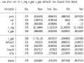
Table 2.3 Testing the stationarity of money supply quantities
Variable
Level | Delay | Value of KĐ | ADF Critical Value Courage 1% 5% 10% | |
M1 | M1 | 1 | 3.8095 | -3.5778 -2.9256 -2.6005 1% Line |
D(1) | 1 | -4.2839 | -3.5814 -2.9271 -2.6013 1% Line | |
M2 | M2 | 1 | 4.9466 | -3.5778 -2.9256 -2.6005 1% Line |
D(1) | 1 | -8.2358 | -3.5814 -2.9271 -2.6013 1% Line | |
DMB | DMB | 1 | 0.8018 | -3.6353 -2.9499 -2.6133 No stop |
D(1) | 1 | -5.7077 | -3.6422 -2.9527 -2.6148 1% Line |
Using the Dickey-Fuller test for unit root testing with the hypothesis H0 is non-stationary, we get the results in Table 2.3. We see that at the 1% significance level, the series M1 and M2 and their first differences are all stationary with a lag of 1. The series DMB is non-stationary, but the first difference series is stationary with a lag of 1 (Appendix E). Thus, we are confident that there will be no spurious regression in the relevant regression results.
Perform regression with the obtained data.
(2.3) | ||
T (-0.014) (15.47)* R 2 = 0.879 F = 239.4 | D – W = 1.315 | |
M1 = 2.549 + 0.917* DMB | (2.4) | |
T (2.77)* (7.26)* R 2 = 0.6304 F = 26.43 | D-W = 2.05 |
(In the results of regression equations, the values in ( ) indicate the value of the T statistic, and the (*), (**) indicate the significance level of 5%, 10%)
In both equations, the coefficient of the available money base is statistically significant at the 5% level. However, in equation (2.3), DMB is a non-stationary series, the intercept is not statistically significant and there is an autocorrelation defect that, when corrected, we obtain a non-stationary process. Equation (2.4) is an equation without these defects. The coefficient of DMB is 0.917, which is statistically significant, indicating that if the available money base increases by 1%, the supply of narrow money will increase by 0.917%. Furthermore, the two series in the regression equation are two stationary series, so there is no spurious regression. The coefficient R2 = 0.6304 can be considered acceptable in models with difference variables. The results show that the increase in the amount of narrow money depends closely on the increase in the available money base.
2.2.4 Determinants of the money multiplier
The determination of the money multiplier m according to the dZ approach mentioned in the previous chapter shows that the factors affecting the money multiplier include the cash ratio, the excess reserve ratio of banks, the deposit ratio and the ratio of other debts. When considering the influence of these factors, it shows that on average during the period under study, these factors contributed to m by 23.1%, (-)43.6%, 2.5% and 44.5% respectively. The contribution of these factors varies from year to year, but in general, they all have a positive influence on m. In particular, in 1999, all factors had a negative influence on
m. The behavior and impact of these factors have been analyzed in monetary theory textbooks ([4], page 210). Therefore, in the following section we will analyze the factors affecting them through empirical models.
2.2.4.1 Ratio between cash usage and demand deposits
The monetary function of demand deposits is limited by the lack of adequate banking services and the habit of the people to use cash in payments. Cash then plays both the role of a medium of exchange and the function of keeping the value of money. The observed data show that the proportion of cash is still too large in the money supply. However, the decline of this proportion over time shows that banking services are being developed. From there we will
Come to consider the factors that influence this ratio.
The cash to demand deposit (C/DD) ratio reflects not only the change between C and DD but also the change beyond that to other assets. Therefore, examining the factors affecting the cash ratio requires identifying the factors that cause the fluctuations in C and DD as well as the fluctuations in
between these two factors. Furthermore, the results of Khatiwada ([89], p. 32) show that the demand for cash as an increasing function of factors such as income,
decrease in the lZi rate and the expected inflation rate. From there we will analyze some of the determinants of cash.
Real income
The results of economists' research show that every increase in real income will reduce the demand for cash if in that economy the payment technique by check is improved ([89], page 33). Therefore, real income
is included as an explanatory variable in the cash ratio function for the following reasons:
- The elasticity of income with respect to cash was found to be significant (Table A12, Appendix A)
- Real income also represents a series of other economic development variables. The higher the economic development, the lower the cash holding ratio among the people, the more effectively people will manage their cash and thus affect the ratio of cash to demand deposits.
Effectiveness of banking services
In developing countries, the efficiency of banks' debt services is an important factor causing the change from cash to demand deposits. The explosion of the banking system caused a great disturbance in payment services and thus increased the shift from cash to demand deposits and term deposits. This proves that the increase in bank branches is a factor that greatly affects the cash ratio. In Vietnam, from having only 4 state-owned banks playing a leading role, by the end of the 90s of the 20th century and the early years of this decade, along with economic development, the development and expansion of the system of commercial banks, commercial banks expanded their networks and improved their operational capacity. In addition, more joint-stock commercial banks were allowed to operate and continuously developed in both scale and level. Unfortunately, we do not have complete data on the development
branches so that the impact of this explanatory variable is considered in the intercept coefficient in the regression equations.
Interest rate
Cash and demand deposits are non-interest bearing assets of the public. Therefore, the opportunity cost of holding these assets is
measured by the deposit rate. If the savings rate increases, time deposits increase, the cash rate will decrease and vice versa. These changes lead to fluctuations in
from cash to time deposits, which affects the secondary money creation of banks. Hence, the coefficient of the input lZi variable is expected to be negative in the regression equations.
Components of income
With the economic renovation policy, economic components have been constantly developing, in which we consider the increase in income in the agricultural production sector as an increase in income in the production establishments of agricultural products, and the increase in income in the non-agricultural production sector is considered as an increase in income of industrial and service production establishments. Therefore, the high growth of income in the agricultural sector will increase the cash ratio and that is a global defect ([89], page 33). GDPNA and GDPAG are two components of GDP income volume. From there, the ratio of agricultural income to total income is
into the regression equation as an explanatory variable with a positive coefficient. However, as the economy develops, the income of the non-agricultural sector will increase faster and account for a very large proportion of total income. Therefore, we will also include this factor in the models as an explanatory variable to examine its impact.
Other factors affecting the cash ratio
During the renovation process, the society has many changes. Factors such as
Table 2.4 Regression results for dependent variable C/DD (1996:1 – 2004:4)
Pt
Number of legs | Q | Dr | GDPAG/GDP | GDPNA/GDP | C/DD(-1) | T | R 2 | F | D –W | |
1 | 1,653 (8.06)* | -0.0022 (-0.97) | 0.0167 (0.74) | -0.652 (-1.32) | - | - | - | 0.896 | 62.89 | 2.56 |
2 | 1.73 (8.83)* | -0.0046 (-3.39)* | 0.0133 (0.58) | - | - | - | - | 0.887 | 81.36 | 2,518 |
3 | 1.54 (8.7)* | - | 0.019 (0.84) | -1.037 (-3.57)* | - | - | - | 0.89 | 83.71 | 2.49 |
4 | 1.81 (6.9)* | -0.0017 (-0.71) | 0.018 (0.78) | -0.74 (-1.43) | - | - | -0.0072 (-0.78) | 0.895 | 49.5 | 2.48 |
5 | 1.8 (6.65)* | -0.0046 (6.65)* | 0.0136 (0.58) | - | -0.0036 (-0.38) | 0.89 | 59.3 | 2.47 | ||
6 | 1.00 (1.72)** | -0.0022 (-1.10) | 0.0168 (0.54) | - | 0.652 (1.32) | - | 0.893 | 62.89 | 2.56 | |
7 | 0.7736 (3.56)* | -0.0043 (2.67)* | 0.6896 (8.97)* | 0.842 | 53.09 | 2.05 | ||||
8 | 0.7078 - 0.0114Dr(-1) – 1.818 GDPAG/GDP + 0.844C/DD(-1) ( 5.44)* (-1.3)** ( -1.82)* (14.02)* | 0.886 | 56.22 | 2,076 | ||||||
9 | 2.129 – 0.0065Q – 0.692 GDPAG/GDP(-1) (10.0)* (-3.45)* (-1.89)** | 0.865 | 64.28 | 2,504 | ||||||
10 | - 0.986 - 0.0139Dr(-1) + 1.836 GDPNA/GDP + 0.799C/DD(-1) - 0.0026T (-2.97)* (-1.64)*** (4.37)* (911.7)* (-1.42)*** | 0.894 | 47.03 | 2,101 | ||||||
Table 2.5 Regression results for dependent variable T&S/DD (1996:1 – 2004:4)
Pt
House choose | Q | Dr | Pe | T&S/DD(-1) | T | R 2 | F | D –W | |
1 | -2.916 (-1.97)** | -0.004 (-1.5)*** | 0.044 (1.12) | 0.035 (3.13)* | - | - | 0.742 | 20.83 | 2.01 |
2 | 2,009 (1.55)*** | -0.005 (-2.19)* | 0.064 (1.67)* | - | - | - | 0.747 | 30.44 | 2,326 |
3 | 2,091 (3.35)* | -0.0048 (-2.03)* | - | - | - | - | 0.724 | 42.03 | 2.39 |
4 | -2.84 (-2.42)* | -0.0059 (-2.3)* | - | 0.037 (3.89)* | - | 0.775 | 35.5 | 2,223 | |
5 | 0.82 (1.02) | -0.005 (-1.78)** | 11.21 (7.77)* | -0.012 (-1.63)*** | - | 0.074 (8.5)* | 0.838 | 40.1 | 1.93 |
6 | 0.559 (2.46)* | -0.0079 (-2.36)* | 0.0295 (1.6)*** | - | 0.558 (4.41)* | 0.026 (4.41)* | 0.817 | 33.4 | 2.26 |
7 | 0.28 (0.32) | -0.0082 (-2.3)* | 0.029 (1.5)*** | 0.0027 (0.32) | 0.559 (4.35)* | 0.0295 (2.9)* | 0.817 | 25.97 | 2.27 |
Note: The values in ( ) are the values of the T-statistic, the (*), (**), (***) indicate the acceptance coefficient with significance levels of 5%, 10%, 15%.