Peak Power to Average Power Ratio (Papr)

Transmitter station

Line 1

Line 2

α 1

Reflective object

Figure 2.11. Transfer function of

2.5.3. AWGN noise

AWGN noise exists in all transmission systems. The main sources of noise are thermal noise, electromagnetic noise from receiver amplifiers, and inter-cell noise. These types of noise can cause inter-symbol interference (ISI) and inter-carrier interference (ICI). This noise reduces the signal-to-noise ratio (SNR), reducing the spectral efficiency of the system. And in fact, depending on the type of application, the noise level and spectral efficiency of the system must be selected.

Most types of noise in systems can be accurately simulated by additive white noise. In other words, Gaussian white noise is the most common type of noise in transmission systems. This type of noise has a power spectral density that is uniform in both bandwidth and amplitude, following a Gaussian distribution. According to the mode of action, Gaussian noise is additive noise. So the common type of transmission channel is the channel affected by additive white Gaussian noise.

2.5.4. Inter-Symbol Interference ISI

ISI (Inter-Symbol interference) is the phenomenon of inter-symbol interference. ISI occurs due to the multi-path effect, in which a later signal will affect the previous symbol. The cause is due to the selectivity of the fading channel in the time domain, the instability of the channel causing signal interference, caused by multi-path delay spread. The effect of ISI: causes wrong recognition of symbols, making it difficult to restore the original signal at the receiver.

To reduce ISI, the best way is to reduce the data rate. But with the current demand, the transmission rate must be increased rapidly. Therefore, this solution is not feasible. The method to reduce ISI and has been put into practical application is to insert a repeating prefix CP into each OFDM symbol.

2.5.5. Inter-carrier interference (ICI)

ICI (Inter-Channel Interference) is cross-channel interference, which is interference caused by signals from adjacent channels interfering with each other. It is inter-cell interference or interference

Inter-cell interference is interference that arises when signals of the same frequency band on different cells in a cellular network interfere with each other.

ICI is a common phenomenon in multicarrier systems. In OFDM systems, ICI, also known as inter-subcarrier interference, is a phenomenon in which the spectral energy of subcarriers overlaps too much, breaking the orthogonality of the subcarriers.

The main cause is the Doppler phenomenon due to the mobility of the transmitter and receiver, there is relative movement between them. Due to the frequency selectivity of the fading channel.

Effect of ICI: subcarriers that lose orthogonality cannot be recovered exactly as transmitted.

2.5.6. Peak power to average power ratio (PAPR)

PAPR is the instantaneous peak power to average power ratio, which is one of the fundamental limitations of OFDM signals. This ratio is expressed by the formula

max s ( t ) 2

math:

PAPR t  [0, T ]

means ( t ) 2

t  [0, T ]

(2.21)

Where s(t) is the multicarrier signal, T is the period of the OFDM symbol.

When this ratio is high, the use of power amplifiers will not be highly efficient because they must reserve power to avoid nonlinear interference. Thus, reducing PAPR is an important requirement of OFDM systems. Figure 2.13 shows that when the carriers are in phase with each other, they will create large peaks, which will cause a very large PAPR ratio.

M-level phase keying (M-PSK) system: because the symbols in the signal space only differ in phase while the magnitude is equal, PAPR = 1. If the PAPR ratio is too large, it will create many disadvantages such as increasing the complexity of the D/A, A/D converter and reducing the efficiency of the high-frequency power supply. Several techniques have been proposed to reduce PAPR. We can divide them into 3 types as follows:

The first is signal distortion techniques. These techniques reduce the peak amplitude simply by distorting the OFDM signal around the signal peak.

Second are coding techniques that use special error-correcting encoders to eliminate OFDM symbols with high PAPR.

Third are techniques based on randomizing each OFDM symbol with

different pseudorandom sequences and choose the one with the smallest PAPR.

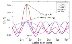
Figure 2.13. Carrier peak appearance

2.6. Advantages and disadvantages of OFDM

2.6.1. Advantages

Bandwidth efficiency

In a conventional FDM system, each sub-channel is separated by a guard space to ensure that adjacent channels do not interfere with each other. Whereas, an OFDM system has overlapping sub-channels. Hence it can make maximum use of the system bandwidth as illustrated in Figure 2.14.

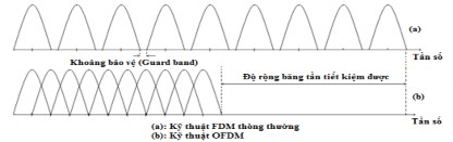
Figure 2.14. Spectrum efficiency of OFDM

Reduce ISI

In single-carrier systems, ISI is often caused by the multipath propagation characteristics of a radio communication channel. In particular, when transmitting a signal over a long distance, the signal is transmitted along many different paths. Therefore, the received signal contains the direct line signal overlapping with the reflected signals with smaller amplitudes, causing signal distortion.

OFDM systems mitigate this problem by creating a symbol interval that is longer than the delay spread of the channel. The signal from a high-speed data stream is divided into N lower-speed data streams. The symbol lifetime of the subchannels is increased by a factor of N , which reduces ISI. Furthermore, ISI can be completely eliminated by adding to the OFDM signal a cyclic preamble (CP) with a sequence length greater than the maximum transmission delay of the channel ∆τ max .

Frequency selective fading reduction and simple system structure

With OFDM system, frequency selective fading only affects one or a few sub-channels with small signal bandwidth, so it can be considered as flat fading. Therefore, the complexity of the equalizer and noise filter is also reduced, allowing the OFDM receiver structure to be much simpler. Furthermore, thanks to the use of corresponding IFFT/FFT converters instead of modulators and demodulators, the transmitter and receiver structures are also much simpler. Especially today, when microchip manufacturing technology develops with high processing speed, OFDM technology is more and more widely applied in information systems, especially in broadband information systems such as WiMAX.

2.6.2. Disadvantages

PAPR ratio

OFDM signals typically have a higher peak-to-average power ratio than single-carrier signals. This is because in the time domain, a multi-carrier signal is the sum of many narrowband signals. In some cases, this sum is large, but in others, it is small, which means that the peak value of the signal is significantly larger than the average value. A high PAPR is one of the biggest challenges of OFDM systems, because it reduces spectral efficiency and pushes the operating point of the power amplifier into the nonlinear region, increasing the cost of the RF ( Radio Frequency ) power amplifier, which is one of the most expensive pieces of equipment in a radio communication system. Therefore, it is necessary to take measures to reduce the PAPR of OFDM signals before they are passed through the power amplifier.

Frequency translation and synchronization

OFDM systems are very sensitive to frequency shift errors because the basic principle of OFDM is that the subcarriers overlap spectrally rather than being spectrally isolated. This frequency shift makes the subcarriers no longer orthogonal to each other, which leads to interference between neighboring subcarriers and causes ICI. Therefore, OFDM systems require very strict frequency synchronization.

CHAPTER III: SPACE-TIME ENCODING

3.1. Introduction

A system with multiple transmit and receive antennas with an independent flat fading channel defined at the receiver has a linear increase in capacity with a minimum number of antennas.

One approach to MIMO channel capacity is to implement space-time coding, a coding technique for implementing multiple transmit antennas. Coding is performed in both the space and time domains to create equivalence between signals transmitted from different antennas at different periods. Space-time equivalence is used to exploit the MIMO channel and minimize transmission errors at the receiver. There are several types of space-time coding, including:

- Space-time block codes (STBC)

- Space-time trellis codes (STTC)

- BLAST (Bell Laboratories Layered Space-Time) layered space-time encoding.

The key to space-time coding is to exploit multipath effects to achieve increased capacity and spectral efficiency.

3.2. STBC block space-time coding

STBC is a simple, efficient diversity technique using two transmit antennas by encoding a block of input symbols into an output matrix with rows corresponding to the transmit antennas. STBC allows full diversity and has small gain depending on the code rate of the encoder, simple decoding, based on ML (Maximum Likelihood) correlation decoders.

3.2.1. Alamouti model

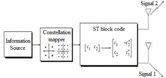
Figure 3.1. Spatial transmit diversity with Alamouti block space-time coding

The Alamouti model is the first model of space-time coding.

The block allows full transmit diversity for the two transmit antennas. However, the receiver must have a complex detector and deal with the problem of inter-symbol interference.

3.2.1.1. Alamouti encoding with two transmit antennas (2 Tx)

The Alamouti cipher block diagram is shown in Figure 3.2.

Tx1

𝑥 1 = 𝑥 1 − 𝑥 ∗

Information Source

𝑥 1 𝑥 2

Encoder

Modulator

𝑥 1 𝑥 2

[

𝑥 1 −𝑥 ∗

Tx2

𝑥 2 = 𝑥 − 𝑥 ∗

𝑥 2

𝑥 ∗

2 ]

2 1

Figure 3.2. Alamouti cipher block diagram

Suppose the binary signal is M-ary modulated. In the Alamouti space-time encoder, each group of m information bits is modulated with 𝑚 = log 2 𝑀 . The encoder then uses an algorithm to encode the two modulated symbols 𝑥 1 and 𝑥 2 into blocks and maps them into a code matrix.

𝑥 1 −𝑥 ∗

𝑋 = [

2 ] (3.1)

𝑥 2 𝑥 ∗

This code matrix is transmitted in two consecutive time intervals on two transmitting antennas. During the first transmission interval, two signals 𝑥 1 and 𝑥 2 are transmitted simultaneously on antennas one and two, respectively. During the second transmission interval, the signal −𝑥 ∗ is transmitted

on the first antenna and 𝑥 ∗ is transmitted on the second antenna, where 𝑥 ∗ is the complex conjugate of 𝑥 1

1 1

as shown in figure 3.3.

It is clear that this encoding is performed on both the spatial and temporal domains.

The transmit chains on the first and second antennas are denoted by 𝑥 1 and 𝑥 2 respectively .

𝑥 1 = ⌊𝑥 1 , −𝑥 ∗ ⌋ (3.2)

𝑥 2 = ⌊𝑥 2 , 𝑥 ∗ ⌋

The special feature of the Alamouti model is that the bit stream is transmitted on two orthogonal transmitting antennas, since the product of the series 𝑥 1 and 𝑥 2 is zero.

𝑥 1 ∙ 𝑥 2 = 𝑥 1 𝑥 ∗ − 𝑥 ∗ 𝑥 1 = 0

Time

Tx 1

Space

c 1

c 2

 c *

c *

c 3

c 4

 c *

c *

c 5

c 6

 c *

c * 5

Maybe you are interested!

T 1 T 2 T 3

T4 T5 T6

r 1

r 2

r 3

r 4

r 5 r6

Rx 1

Figure 3.3. Transmission and reception symbols of the Alamouti model

The code matrix has the following properties:

𝐻 |𝑥 1 | 2 + |𝑥 2 | 2 0 2 2

𝑋. 𝑋 = [

0 |𝑥 1

| 2 + |𝑥 2

| 2 ] = (|𝑥 1 |

+ |𝑥 2 |

)𝐼 2 (3.3)

Where I 2 is a 2x2 identity matrix.

Data

Tx 1

h 1

x 2

 nn 

1 2

Combination set

ML Decoder

Space-Time encoder  c c *  cc   1 2  1 2   c c *  2 1
	T

~ r

	H
Estimate
Estimate		H

h 2

Figure 3.4. Alamouti diagram with two transmitting antennas and two receiving antennas

Assume that the receiver uses only one receiving antenna. The block diagram of the receiver for the Alamouti model is shown in Figure 3.4. The fading coefficients from the first and second antennas to the receiver at time t are denoted by ℎ 1 (𝑡) and ℎ 2 (𝑡) respectively. Assuming that the fading coefficients are constant over two consecutive transmission intervals, these coefficients are expressed as

ℎ 1 (𝑡) = ℎ 1 (𝑡 + 𝑇) = ℎ 1 = |ℎ 1 |𝑒 𝑗𝜃 1 (3.4)

ℎ 2 (𝑡) = ℎ 2 (𝑡 + 𝑇) = ℎ 2 = |ℎ 2 |𝑒 𝑗𝜃 2

Transmit Antenna 1

𝑥 1

−𝑥 ∗

Transmit Antenna 2

Where, |ℎ 𝑖 | and 𝜃 𝑖 , 𝑖 = 0, 1, are the amplitude gain and phase shift for the transmission path from the transmitting antenna i to the receiving antenna , and T is the symbol length.

𝑥 2

−𝑥 ∗

Receive antenna

𝑛 1 , 𝑛 2

+ noise

ℎ 1

Channel Estimator

ℎ 2

Signal Combiner

ℎ 1

ℎ 2

𝑥 1

𝑥 2

Maximum Likelihood Decoder

𝑥 1

𝑥 2

Figure 3.5. Receiver of the Alamouti model

At the receiving antenna, the signal receives two consecutive symbol intervals, denoted as 𝑟 1 and 𝑟 2 for times 𝑡 and 𝑡 + 𝑇 , respectively, described as follows

𝑟 1 = ℎ 1 𝑥 1 + ℎ 2 𝑥 2 + 𝑛 1 (3.5)

𝑟 2 = −ℎ 1 𝑥 ∗ + ℎ 2 𝑥 ∗ + 𝑛 2

2 1

Where, 𝑛 1 and 𝑛 2 are free complex variables with zero mean and power spectral density 𝑁 0 /2 , which are white Gaussian additive noise samples at times 𝑡 and 𝑡 + 𝑇 , respectively

3.2.1.2. Combining and maximum likelihood decoding

If the fading channel coefficients, ℎ 1 (𝑡) and ℎ 2 (𝑡) can be fully recovered at the receiver, the encoder can use them as channel state information (CSI). Assuming that all signals in the modulation constellation have equal probability, the maximum correlation encoder selects a pair of signals (𝑥 1 , 𝑥 2 ) from the signal modulation constellation to minimize the metric distance as formula (3.5)

Substituting 𝑟 1 and 𝑟 2 from (3.4) into (3.5), the maximum correlation decoder is represented as follows:

𝑑 2 (𝑟 1 , ℎ 1 𝑥 1+ ℎ 2 𝑥 2 ) + 𝑑 2 (𝑟 2 , −ℎ 1 𝑥 ∗+ ℎ 2 𝑥 ∗ )

2 1

= |𝑟 1− ℎ 1 𝑥 1− ℎ 2 𝑥 2 | 2+ |𝑟 2+ ℎ 1 𝑥 ∗− ℎ 2 𝑥 ∗ | 2

2 1

2 2 2 2 2 2

(𝑥 1 , 𝑥 2 ) = arg min (𝑥1 , 𝑥 2 )∈ 𝐶 (|ℎ 1 | + |ℎ 2 | − 1)(|𝑥 1 | + |𝑥 2 | ) + 𝑑 (𝑥 1 , 𝑥 1 ) 𝑑 (𝑥 2 , 𝑥 2 )

(3.6)

In which, C is the set of modulation symbol pairs (𝑥 1 , 𝑥 2 ) , 𝑥 1 , 𝑥 2are two statistical decisions calculated by combining the received signals with the transmission channel given by the formula:

𝑥 1 = ℎ ∗ 𝑟 1 + ℎ 2 𝑟 ∗ (3.7)

1 2

𝑥 2 = ℎ ∗ 𝑟 1 + ℎ 1 𝑟 ∗

2 2

Substituting 𝑟 1 and 𝑟 2 into (3.7), the statistical decision is rewritten as follows:

𝑥 1 = (|ℎ 1 | 2 + |ℎ 2 | 2 )𝑥 1 + ℎ ∗ 𝑛 1 + ℎ 2 𝑛 ∗(3.8)

1 2

𝑥 2 = (|ℎ 1 | 2 + |ℎ 2 | 2 )𝑥 2 − ℎ 1 𝑛 ∗ +ℎ ∗ 𝑛 1

2 2

Given real ℎ 1 and ℎ 2 , the statistical decision, .., 𝑖 = 1,2 are just functions of 𝑥 𝑖 ,

𝑖 = 1.2 . Therefore, the maximum correlation decoding rule can be divided into two independent decoding rules for 𝑥 1 and 𝑥 2 respectively by the formula (3.9) below:

𝑥 1= arg min 𝑥1 ∈ 𝑆 (|ℎ 1 | 2+ |ℎ 2 | 2− 1)|𝑥 1 | 2+ 𝑑 2 (𝑥 1 , 𝑥 1 ) (3.9)