Correlation Coefficient Results and Significance Level of Correlation Coefficient Test for Joint Stock Commercial Bank Group

3.3.3.3. Testing the simple regression coefficient

Simple regression coefficient test Hypothesis: H 0 : β i = 0

H 1 : β i ≠ 0, where k is the number of variables in the model

, with significance level α if sig.  α then we reject H 0 and accept H 1 .

Table 3.14: Single regression coefficient test

Coefficients

Looking at the regression results table, we see that all Sig. values ​​are less than α=10% or all t values ​​are statistically significant with a significance level of α=10% (ie the confidence level is 90%), we can conclude that the above three factors all have an impact on the ROA fluctuations of the joint stock commercial banking system with a confidence level of 90%.

3.3.3.4. Multicollinearity test

Table 3.15: Multicollinearity test

Coefficients

The results of the table above show that the VIF (Variance inflation Factor) is very small, all values ​​are less than 3, and a VIF value of less than 10 is considered to have no significant multicollinearity, so it can be concluded that the correlation between independent variables does not significantly affect the explanatory ability of the regression model of the joint stock commercial banking system.

3.3.3.5. Autocorrelation test

The regression result of model (2) has a Durbin-Waston coefficient of 2.555 (table 3.17) which is still in the range of 1 to 3, so according to Willson & Keating (2002), we can conclude that there is no significant autocorrelation between the variables in the model.

3.3.3.6. Test for normal distribution

 Histogram to examine normal distribution

Figure 3.5: Histogram

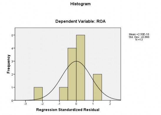
Based on the chart above, it shows that the Mean value is very small, close to 0.000, and the standard deviation Std.Dev.=0.866 - close to the normal distribution. Therefore, it can be concluded that the normal distribution hypothesis is not violated when applying the OLS linear regression method.

 PP Plot frequency chart examines normal distribution.

Chart 3.6: PP Plot Frequency Histogram

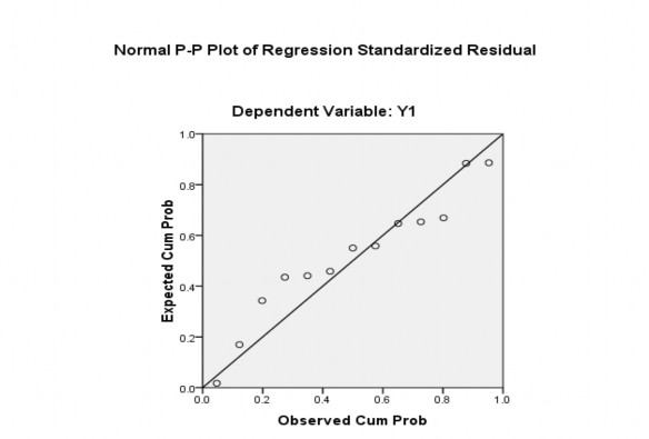
By observing the actual points scattered around the expected line, the above graph shows that the scattered points are not too far from the expected line so it can be concluded that the normal distribution hypothesis is not violated.

 Kolmogorov-Smirnov test for normally distributed residuals Hypothesis H 0 : residuals are normally distributed

H 1 : residuals are not normally distributed

If the Sig. value > significance level α then the null hypothesis H 0 is not rejected.

Table 3.16: Kolmogorov-Smirnov test

Kolmogorov-Smirnov test gives the result with Sig.= 0.708, much larger than the significance level α= 10% so the hypothesis H 0 cannot be rejected even with only 90% confidence, therefore we accept the hypothesis H 0 , it can be concluded that the residuals are normally distributed.

3.5.1.1 Estimating the coefficient of determination and assessing the model's suitability

The calculation formula, meaning of the coefficient of determination; basis and criteria for evaluating the suitability of the regression model have been stated in section 3.5.2.8. Based on the above theoretical basis, consider the indicators in the table below.

Table 3.17: Estimated coefficient of determination and model fit assessment.

Model Summary

With the coefficient R 2 (R Square) equal to 0.832, it shows that the regression model fits well with the database or the independent factors in the model explain 83.2% of the change in the dependent variable Y 1 . The model's suitability is high.

3.5.1.2 Estimating regression coefficients in the model

Table 3.18: Estimated regression results

Coefficients

Based on the regression results in the table above, we get the following regression model:

Y 1 = 0.031 – 0.038X 8 + 0.104X 10 – 0.780X 12 (2) Std = (0.015) (0.018) (0.031) (0.202)

t = (2.090) (-2.124) (3.327) (-3.853)

Sig. = (0.066) (0.063) (0.009) (0.004)

N=13; R 2 = = 0.832; F = 14,810;

With: X 8 is the ratio of interest income/Total income, X 10 is the ratio of foreign currency loans/Total loans, X 12 is Foreign currency assets/Total capital.

Unstandardized regression coefficient (denoted B in Table 3.18): partial regression coefficient measures the change in the mean value of the dependent variable (Y 1 ) when an independent variable (X 8 , or X 10 , or X 12 ) changes by one unit, provided that the remaining independent variables in the model remain unchanged. In which, a positive regression coefficient shows a positive change in the dependent variable when the independent variable increases/decreases, and a negative regression coefficient shows that the dependent variable will change in the opposite direction to the change in the influencing factor.

Economic significance of regression models

Based on the results of Table 3.18 (beta coefficient), it shows that the variable with the strongest impact on the performance of the group of joint stock commercial banks is factor X 12 (Foreign currency liabilities/Total capital), followed by factor X 10 (ratio of foreign currency loans/Total loans), and finally the factor with the lowest impact is X 8 (ratio of interest income/Total income).

When the ratio of Interest Income/Total Income is in the range (0.7369; 0.9400) and under the condition that other factors remain unchanged, if the ratio of interest income/total income increases/decreases by 1 unit, the return on total assets (ROA) will decrease/increase by 0.038 units with a significance level of α= 10%, so to increase the efficiency of the commercial banking system according to the above model means reducing the ratio of interest income to total income.

When the ratio of foreign currency loans/total outstanding loans is within the range (0.1383; 0.2239) and under the condition that other factors remain unchanged, if the ratio of foreign currency loans/total outstanding loans increases/decreases by 1 unit, ROA (the efficiency of the joint stock commercial banking system) increases/decreases by 0.104 units; therefore, the above model gives the result that if banks want to increase ROA, they should increase foreign currency loans.

With the ratio of foreign currency debt assets/Total capital in the range of (0.0002; 0.0164) and under the condition that other factors remain unchanged, if the ratio of foreign currency debt assets/Total capital increases/decreases by 1 unit, the bank's efficiency decreases/increases by 0.780 units, so to increase efficiency