Assessing the Impact of Quality of Work Life on Work Performance – Model 1

In which, the Existence Need Satisfaction factor has the strongest correlation (Person correlation coefficient is 0.748), the Relationship Need Satisfaction factor has the weakest correlation (Person correlation coefficient is 0.715).

At the same time, the analysis results also show that there is a correlation between Job Performance and the independent variables Existence Need Satisfaction, Relationship Need Satisfaction, and Knowledge Need Satisfaction, and this relationship is close. In which, the Existence Need Satisfaction factor has the strongest correlation (Person correlation coefficient is 0.766), the Relationship Need Satisfaction factor has the weakest correlation (Person correlation coefficient is 0.735).

The relationship between Job Satisfaction and Job Performance is a close relationship, the Person correlation coefficient is up to 0.986.

So in general, with a significance level of 1%, there is a correlation between the independent variables. The closer this value is to 1, the higher the linear relationship, /r/ > 0.8 shows a very strong linear relationship, which also means that there is multicollinearity between these variables. To clarify the multicollinearity phenomenon, the topic will use the VIF coefficient to test the assumptions in the next section.

The study has the following regression models:

Model 1: Assessing the impact of quality of work life on employee performance. The factors TT, QH, KT are independent variables, and the factor KQ is the dependent variable.

KQ = β 0 + β 1 TT + β 2 QH + β 3 KT

Model 2: Assessing the impact of quality of work life on employee job satisfaction. TT, QH, KT are independent variables, HL is the dependent variable.

HL = β 0 ' + β 4 TT + β 5 QH + β 6 KT

4.2.2 Regression analysis

4.1.2.1 Assessing the impact of quality of work life on work performance – model 1 - The impact of quality of work life on job satisfaction

a. Model building

Model KQ = β 0 + β 1 TT + β 2 QH + β 3 KT . Using SPSS 16 software. Build and evaluate the impact of quality of work life on employee work performance using the Enter method. In which, factors TT, QH, KT are independent variables, KQ is dependent variable. The results are presented in Appendix 7 - results of regression model 1 analysis.

To assess the model's fit, researchers use the coefficient of determination R 2 (R-square) to assess the fit of the research model. The coefficient of determination R 2 has been shown to not necessarily increase with the number of independent variables added to the model, however, not all equations with more variables will fit the data better, R 2 tends to be an optimistic factor of the measure of the model's fit to the data in the case of a number of explanatory variables in the model. Thus, in multiple linear regression, the adjusted R 2 coefficient is often used to assess the fit of the model because it does not inflate the fit of the model.

The adjusted R 2 regression result is 0.829, meaning that the model explains 82.9% of the variation in the job satisfaction variable, for the model of the influence of quality of work life on job satisfaction; and in the model of the influence of quality of work life on job performance, the adjusted R 2 regression result is 0.829, meaning that the model explains 82.9% of the variation.

of the job outcome variables and the above models fit the data at the 95% confidence level.

Table 4.4 Results of regression parameters of model 1

Model

	Unstandardized coefficient		Coefficient standardize	t-test	Significance level (Sig.)	Multicollinearity statistics line
	Regression coefficient (β)	Standard error	Regression coefficient (β)	t-test	Significance level (Sig.)	Acceptability	Magnification factor wrong (VIF)
1	Constant	0.732	0.115		6,346	0.000
	TT	0.299	0.028	0.392	10,565	0.000	0.623	1,604
	QH	0.306	0.027	0.387	11,114	0.000	0.706	1,417
	KT	0.258	0.029	0.333	8,953	0.000	0.620	1,614

Maybe you are interested!

Dependent variable: Result

(Source: SPSS results)

The results of the regression analysis show that all three factors of the quality of work life scale have an impact on work outcomes (because the Sig of the regression weights all reach the significance level). On the other hand, because the Beta coefficients are all positive, these variables all have a positive impact on work outcomes.

Model 1 is rewritten with unstandardized coefficients:

Result = 0.732 + 0.299 *TT+0.306*QH+0.258KT or:

Quality of work life = 0.732 + 0.299 * (Existence needs satisfaction) + 0.306 * (Relationship needs satisfaction) + 0.258 * (Knowledge needs satisfaction). So:

To determine the level of influence of the factors TT, QH, KT on KQ, we base on the Beta coefficient. The larger the Beta, the higher the level of influence on KQ and vice versa. Under the condition that the factors QH (Satisfaction of relationship needs) and KT (Satisfaction of knowledge needs) remain unchanged, the factor TT (Satisfaction of existence needs) increases by 1 unit on the Likert scale, KQ (Work results) will increase by 0.299 units on the Likert scale. And the hypothesis:

H1a: Existence need satisfaction has a positive impact on work performance: ACCEPTANCE

Similar reasoning is used for the QH factors (Satisfaction of relationship needs) and the KT factor (Satisfaction of knowledge needs). The following hypotheses are accepted:

H1b: Satisfaction of relationship needs has a positive impact on job performance.

job

H1c: Satisfaction of knowledge needs has a positive impact on performance

job

Model 1 is written in terms of standardized coefficients:

Job performance = 0.392 * (Existence need satisfaction) + 0.387 * (Relationship need satisfaction + 0.333 * (Knowledge need satisfaction)

b. Check the assumptions of OLS regression

- Constant variance of residuals and linear relationship: the study uses Scatterplot of standardized residuals and standardized predicted values. Observing the graph, we see that the residuals are randomly scattered around the 0 axis and do not create any specific shape (Appendix - Scatterplot 1), that is, around the mean value of the residuals within a constant range. This means that the variance of the residuals is constant and there is a linear relationship between KQ and the independent variables.

Figure 4.1 Scatterplot 1 – Scatterplot between residuals and predicted values

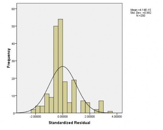
- The residuals are normally distributed: the Histogram of the standardized residuals will test this assumption. We see that the normal distribution curve is superimposed on the histogram and is considered as approximately normally distributed residuals and the assumption of normally distributed residuals is not violated. From the Histogram of the standardized residuals, it shows that the distribution of the residuals is approximately normal (Mean=0, Std.Dev=0.992) (Appendix 8 - Histogram of standardized residuals 1). This leads to the conclusion that the assumption of normal distribution of the residuals is not violated.

Figure 4.2 Histogram 1 – Frequency of standardized residuals

- Assume there is no correlation between independent variables: that is, check for multicollinearity. If multicollinearity occurs, the tolerance of the variable will be very small or the VIF variance magnification factor will be large. (According to Hoang & Chu 2005, 2008, VIF>5 will cause multicollinearity, according to Nguyen 2011, VIF>2 will cause multicollinearity). The results show that the tolerance of the large and smallest variable is 1.417 and the smallest and largest VIF coefficient is 1.614<2 (Appendix 7 - Regression weight table 1). So there is no multicollinearity in the multiple regression model.

Conclusion: Regression model 1: suitable for the data set, suitable for the population, coefficients β 1, β 2, β 3 are statistically significant, there is no multicollinearity between independent variables, no violation of linearity assumption, residual assumption such as constant variance, normal distribution and independence. Hypotheses H1a, H1b, H1c are accepted.

4.1.2.2 Assessing the impact of quality of work life on job satisfaction of bank employees – model 2

a. Model building

Similar to above, using SPSS 16 software: Build and evaluate the impact of quality of work life on job satisfaction of employees using the Enter method. In which, the factors TT, QH, KT are independent variables, HL is the dependent variable. The results are presented in Appendix 6 - results of regression model analysis 2.

The adjusted R 2 regression result is 0.795, which means that the model explains

79.5% of the variation in job satisfaction variable, for the model of the influence of quality of work life on job satisfaction, the above model fits the data at 95% confidence level.

Model 2: The impact of quality of work life on job satisfaction

Table 4.5 Results of regression parameters of model 2

Model

	Unstandardized coefficient chemical		Standard coefficient chemical	t-test	Significance level (Sig.)	Multicollinearity statistics line
	Regression coefficient (β)	Standard error	Regression coefficient (β)	t-test	Significance level (Sig.)	Acceptability	Magnification factor wrong (VIF)
2	Constant	0.733	0.129		5,702	0.000
	TT	0.293	0.032	0.377	9,287	0.000	0.623	1,604
	QH	0.297	0.031	0.370	9,690	0.000	0.706	1,417
	KT	0.269	0.032	0.342	8,391	0.000	0.620	1,614

Dependent variable: HL

Model 2 is rewritten with unstandardized coefficients:

(Source: SPSS results)

HL= 0.733 + 0.293 * TT+0.297 * QH+0.269 * KT or:

Job satisfaction = 0.733 + 0.293 * (Existence needs satisfaction)

+ 0.297 * (Satisfaction of relationship needs) + 0.269 * (Satisfaction of knowledge needs). So:

Under the condition that the factors QH (Satisfaction of relationship needs) and KT (Satisfaction of knowledge needs) remain unchanged, the factor TT (Satisfaction of existence needs) increases by 1 unit on the Likert scale, then HL (Job satisfaction) will increase by 0.293 units on the Likert scale. And the hypothesis:

H2a: Existence need satisfaction has a positive impact on job satisfaction: ACCEPTANCE

Similar reasoning is used for the QH factors (Satisfaction of relationship needs) and the KT factor (Satisfaction of knowledge needs). The following hypotheses are accepted:

H2b: Satisfaction of relationship needs has a positive impact on job satisfaction

H2c: Satisfaction of knowledge needs has a positive impact on job satisfaction

Model 2 is written in terms of standardized coefficients:

Job satisfaction = 0.377 * (Existence need satisfaction) + 0.370 * (Relationship need satisfaction) + 0.342 * (Knowledge need satisfaction)

c. Check the assumptions of OLS regression

Testing the assumption similar to model 1, we have the Scatterplot and Histogram in the SPSS run results of model 2 showing that the acceptability of the largest variable, the smallest reaches 1.417 and the smallest VIF coefficient, the largest reaches 1.614<2 (Appendix 6 - Regression weight table 2). So there is no multicollinearity in the multiple regression model.

Detect violations of model assumptions:

- Linearity violation assumption: through the graph below, it can be seen that this assumption is rejected because the standardized residuals are completely randomly distributed.

Assessing the Impact of Quality of Work Life on Work Performance – Model 1 - Impact of Quality of Work Life

Comment