- Using BT in general, and BT in Educationin particular, needs to take into account the space for implementation (in class, outside class), teaching time for each subject, and each lesson. BT at home needs to ensure time for students to be able to do it. In addition, teachers need to spend time checking students' self-study results through personal BT notebooks to have comprehensive comments on students' learning results for each subject. Practical experience shows that: Where teachers regularly check students' learning, there students' learning awareness and learning results are better.
* For students : With the current credit training method at universities, the concept of a classroom is only relative. For general subjects, students from different faculties often study together, so the number of students in theory hours is often large, around 150 - 200 students, even up to 300 students in some classes. For discussion hours, depending on each school, the number of students/discussion class is regulated, usually only after more than 80 students are divided into groups, so teachers will encounter many difficulties in individualizing teaching and controlling students' learning outcomes . To study effectively, students need to proactively plan their own self-study, be self-aware, positive, and independently solve learning tasks in many different ways, need to find new ways, optimal solutions, and be highly creative.
Chapter 3 Conclusion
1. Activating students' learning activities is the process of using teaching methods to affect students' learning process, changing the position of students in the learning process, from being a passive recipient of knowledge, to becoming a self-conscious, active, and self-reliant subject carrying out the learning process through solving learning tasks to achieve the set goals. To activate students' learning activities in the subject of Education, lecturers can use many measures. One of the measures with high practical significance is the use of the BT system in teaching. The use of BT can be carried out in all class hours, teachers not only use it during class but also guide students to study at home, use BT in testing and evaluating the learning outcomes of the subject.
2. Inheriting research results of domestic and foreign scientists,
We have researched and perfected the theoretical basis for designing and using BT in
The lessons (theory, discussion /seminars, self-study) include requirements , principles,
The process of designing and using exercises . The basic content of this theory has practical significance , helping teachers to refer to when designing and using exercises in teaching. Although each subject has its own characteristics, when designing exercises, it is necessary to take into account specific requirements, but in general, it is still necessary to follow a certain process to achieve high results in teaching.
3. Based on the analysis of the content and duration of each chapter in the Pedagogy course, we have planned the number of exercises and types of exercises, ensuring the balance between theoretical exercises - discussion exercises, reenactment exercises - creative exercises.
Based on the process of designing the training system, we designed the training system part I: " General issues in education" . Applying the process of using training systems, we illustrated the use of training systems in class hours (theory, discussion/semiosis, self-study) as a source of materials for teachers to refer to in teaching.
Designing and using exercises in subjects in general, and Education in particular, is a suitable teaching direction in universities, which needs to be widely disseminated and encouraged for lecturers to apply, because creating and using the BT system in teaching will foster learners' ability to think independently, creatively, and train and form lifelong learning skills in learners.
4. To design and use the general teaching system, and the teaching system in particular, effectively, it is necessary to ensure certain conditions , including objective and subjective conditions . The combination of these conditions aims to contribute to improving the quality of teacher training in pedagogical universities today .
Chapter 4
PEDAGOGICAL EXPERIMENT
4.1. General overview of the experimental process
4.1.1. Experimental purpose
The pedagogical experiment aims to verify the effectiveness of the BT usage process and the designed BT system, thereby fostering students ' positive attitudes towards the subject in teaching GDDH.
4.1.2. Experimental content
The experiment uses the designed BT system in the teaching process of chapters II and III of the pedagogical subject: Education and personality development, purpose and tasks of education . The experimental content is compiled into lesson plans through class hours (theory, discussion, self-study) and implemented according to the BT usage process analyzed in chapter III (section 3.2.3) to practice the skills: problem recognition; data screening, hypothesis building ; problem solving skills; testing and evaluation skills of students' performance.
To accurately and objectively reflect the experimental results, after finishing chapter I, we let students of the experimental and control classes take the same test to evaluate the input quality before conducting the experiment.
4.1.3. Experimental subjects
Are second- year students of the University of Education and first-year students of the College of Education , Hong Duc University , Thanh Hoa. The pedagogical experiment was conducted in two rounds in two school years, in the form of controlled experiments. The experimental subjects were randomly selected according to the teaching assignment . Specifically as follows:
- Experimental round 1: school year 2010 - 2011
Table 4.1: Experimental subjects
System
Class | Object | Symbol | Number of students | |
University | K12 Math | Experiment | TN 1 | 43 |
K12 English | Control | DC 1 | 34 | |
CD | K32 Math - IT | Experiment | TN 2 | 77 |
K32 English | Control | DC 2 | 53 |
Maybe you are interested!
-
![Qos Assurance Methods for Multimedia Communications
zt2i3t4l5ee
zt2a3gs
zt2a3ge
zc2o3n4t5e6n7ts
low. The EF PHB requires a sufficiently large number of output ports to provide low delay, low loss, and low jitter.
EF PHBs can be implemented if the output ports bandwidth is sufficiently large, combined with small buffer sizes and other network resources dedicated to EF packets, to allow the routers service rate for EF packets on an output port to exceed the arrival rate λ of packets at that port.
This means that packets with PHB EF are considered with a pre-allocated amount of output bandwidth and a priority that ensures minimum loss, minimum delay and minimum jitter before being put into operation.
PHB EF is suitable for channel simulation, leased line simulation, and real-time services such as voice, video without compromising on high loss, delay and jitter values.
Figure 2.10 Example of EF installation
Figure 2.10 shows an example of an EF PHB implementation. This is a simple priority queue scheduling technique. At the edges of the DS domain, EF packet traffic is prioritized according to the values agreed upon by the SLA. The EF queue in the figure needs to output packets at a rate higher than the packet arrival rate λ. To provide an EF PHB over an end-to-end DS domain, bandwidth at the output ports of the core routers needs to be allocated in advance to ensure the requirement μ > λ. This can be done by a pre-configured provisioning process. In the figure, EF packets are placed in the priority queue (the upper queue). With such a length, the queue can operate with μ > λ.
Since EF was primarily used for real-time services such as voice and video, and since real-time services use UDP instead of TCP, RED is generally
not suitable for EF queues because applications using UDP will not respond to random packet drop and RED will strip unnecessary packets.
2.2.4.2 Assured Forwarding (AF) PHB
PHB AF is defined by RFC 2597. The purpose of PHB AF is to deliver packets reliably and therefore delay and jitter are considered less important than packet loss. PHB AF is suitable for non-real-time services such as applications using TCP. PHB AF first defines four classes: AF1, AF2, AF3, AF4. For each of these AF classes, packets are then classified into three subclasses with three distinct priority levels.
Table 2.8 shows the four AF classes and 12 AF subclasses and the DSCP values for the 12 AF subclasses defined by RFC 2597. RFC 2597 also allows for more than three separate priority levels to be added for internal use. However, these separate priority levels will only have internal significance.
PHB Class
PHB Subclass
Package type
DSCP
AF4
AF41
Short
100010
AF42
Medium
100100
AF43
High
100110
AF3
AF31
Short
011010
AF32
Medium
011100
AF33
High
011110
AF2
AF21
Short
010010
AF22
Medium
010100
AF23
High
010110
AF1
AF11
Short
001010
AF12
Medium
001100
AF13
High
001110
Table 2.8 AF DSCPs
The AF PHB ensures that packets are forwarded with a high probability of delivery to the destination within the bounds of the rate agreed upon in an SLA. If AF traffic at an ingress port exceeds the pre-priority rate, which is considered non-compliant or “out of profile”, the excess packets will not be delivered to the destination with the same probability as the packets belonging to the defined traffic or “in profile” packets. When there is network congestion, the out of profile packets are dropped before the in profile packets are dropped.
When service levels are defined using AF classes, different quantity and quality between AF classes can be realized by allocating different amounts of bandwidth and buffer space to the four AF classes. Unlike
EF, most AF traffic is non-real-time traffic using TCP, and the RED queue management strategy is an AQM (Adaptive Queue Management) strategy suitable for use in AF PHBs. The four AF PHB layers can be implemented as four separate queues. The output port bandwidth is divided into four AF queues. For each AF queue, packets are marked with three “colors” corresponding to three separate priority levels.
In addition to the 32 DSCP 1 groups defined in Table 2.8, 21 DSCPs have been standardized as follows: one for PHB EF, 12 for PHB AF, and 8 for CSCP. There are 11 DSCP 1 groups still available for other standards.
2.2.5.Example of Differentiated Services
We will look at an example of the Differentiated Service model and mechanism of operation. The architecture of Differentiated Service consists of two basic sets of functions:
Edge functions: include packet classification and traffic conditioning. At the inbound edge of the network, incoming packets are marked. In particular, the DS field in the packet header is set to a certain value. For example, in Figure 2.12, packets sent from H1 to H3 are marked at R1, while packets from H2 to H4 are marked at R2. The labels on the received packets identify the service class to which they belong. Different traffic classes receive different services in the core network. The RFC definition uses the term behavior aggregate rather than the term traffic class. After being marked, a packet can be forwarded immediately into the network, delayed for a period of time before being forwarded, or dropped. We will see that there are many factors that affect how a packet is marked, and whether it is forwarded immediately, delayed, or dropped.
Figure 2.12 DiffServ Example
Core functionality: When a DS-marked packet arrives at a Diffservcapable router, the packet is forwarded to the next router based on
Per-hop behavior is associated with packet classes. Per-hop behavior affects router buffers and the bandwidth shared between competing classes. An important principle of the Differentiated Service architecture is that a routers per-hop behavior is based only on the packets marking or the class to which it belongs. Therefore, if packets sent from H1 to H3 as shown in the figure receive the same marking as packets from H2 to H4, then the network routers treat the packets exactly the same, regardless of whether the packet originated from H1 or H2. For example, R3 does not distinguish between packets from h1 and H2 when forwarding packets to R4. Therefore, the Differentiated Service architecture avoids the need to maintain router state about separate source-destination pairs, which is important for network scalability.
Chapter Conclusion
Chapter 2 has presented and clarified two main models of deploying and installing quality of service in IP networks. While the traditional best-effort model has many disadvantages, later models such as IntServ and DiffServ have partly solved the problems that best-effort could not solve. IntServ follows the direction of ensuring quality of service for each separate flow, it is built similar to the circuit switching model with the use of the RSVP resource reservation protocol. IntSer is suitable for services that require fixed bandwidth that is not shared such as VoIP services, multicast TV services. However, IntSer has disadvantages such as using a lot of network resources, low scalability and lack of flexibility. DiffServ was born with the idea of solving the disadvantages of the IntServ model.
DiffServ follows the direction of ensuring quality based on the principle of hop-by-hop behavior based on the priority of marked packets. The policy for different types of traffic is decided by the administrator and can be changed according to reality, so it is very flexible. DiffServ makes better use of network resources, avoiding idle bandwidth and processing capacity on routers. In addition, the DifServ model can be deployed on many independent domains, so the ability to expand the network becomes easy.
Chapter 3: METHODS TO ENSURE QoS FOR MULTIMEDIA COMMUNICATIONS
In packet-switched networks, different packet flows often have to share the transmission medium all the way to the destination station. To ensure the fair and efficient allocation of bandwidth to flows, appropriate serving mechanisms are required at network nodes, especially at gateways or routers, where many different data flows often pass through. The scheduler is responsible for serving packets of the selected flow and deciding which packet will be served next. Here, a flow is understood as a set of packets belonging to the same priority class, or originating from the same source, or having the same source and destination addresses, etc.
In normal state when there is no congestion, packets will be sent as soon as they are delivered. In case of congestion, if QoS assurance methods are not applied, prolonged congestion can cause packet drops, affecting service quality. In some cases, congestion is prolonged and widespread in the network, which can easily lead to the network being frozen, or many packets being dropped, seriously affecting service quality.
Therefore, in this chapter, in sections 3.2 and 3.3, we introduce some typical network traffic load monitoring techniques to predict and prevent congestion before it occurs through the measure of dropping (removing) packets early when there are signs of impending congestion.
3.1. DropTail method
DropTail is a simple, traditional queue management method based on FIFO mechanism. All incoming packets are placed in the queue, when the queue is full, the later packets are dropped.
Due to its simplicity and ease of implementation, DropTail has been used for many years on Internet router systems. However, this algorithm has the following disadvantages:
− Cannot avoid the phenomenon of “Lock out”: Occurs when 1 or several traffic streams monopolize the queue, making packets of other connections unable to pass through the router. This phenomenon greatly affects reliable transmission protocols such as TCP. According to the anti-congestion algorithm, when locked out, the TCP connection stream will reduce the window size and reduce the packet transmission speed exponentially.
− Can cause Global Synchronization: This is the result of a severe “Lock out” phenomenon. Some neighboring routers have their queues monopolized by a number of connections, causing a series of other TCP connections to be unable to pass through and simultaneously reducing the transmission speed. After those monopolized connections are temporarily suspended,
Once the queue is cleared, it takes a considerable amount of time for TCP connections to return to their original speed.
− Full Queue phenomenon: Data transmitted on the Internet often has an explosion, packets arriving at the router are often in clusters rather than in turn. Therefore, the operating mechanism of DropTail makes the queue easily full for a long period of time, leading to the average delay time of large packets. To avoid this phenomenon, with DropTail, the only way is to increase the routers buffer, this method is very expensive and ineffective.
− No QoS guarantee: With the DropTail mechanism, there is no way to prioritize important packets to be transmitted through the router earlier when all are in the queue. Meanwhile, with multimedia communication, ensuring connection and stable speed is extremely important and the DropTail algorithm cannot satisfy.
The problem of choosing the buffer size of the routers in the network is to “absorb” short bursts of traffic without causing too much queuing delay. This is necessary in bursty data transmission. The queue size determines the size of the packet bursts (traffic spikes) that we want to be able to transmit without being dropped at the routers.
In IP-based application networks, packet dropping is an important mechanism for indirectly reporting congestion to end stations. A solution that prevents router queues from filling up while reducing the packet drop rate is called dynamic queue management.
3.2. Random elimination method – RED
3.2.1 Overview
RED (Random Early Detection of congestion; Random Early Drop) is one of the first AQM algorithms proposed in 1993 by Sally Floyd and Van Jacobson, two scientists at the Lawrence Berkeley Laboratory of the University of California, USA. Due to its outstanding advantages compared to previous queue management algorithms, RED has been widely installed and deployed on the Internet.
The most fundamental point of their work is that the most effective place to detect congestion and react to it is at the gateway or router.
Source entities (senders) can also do this by estimating end-to-end delay, throughput variability, or the rate of packet retransmissions due to drop. However, the sender and receiver view of a particular connection cannot tell which gateways on the network are congested, and cannot distinguish between propagation delay and queuing delay. Only the gateway has a true view of the state of the queue, the link share of the connections passing through it at any given time, and the quality of service requirements of the
traffic flows. The RED gateway monitors the average queue length, which detects early signs of impending congestion (average queue length exceeding a predetermined threshold) and reacts appropriately in one of two ways:
− Drop incoming packets with a certain probability, to indirectly inform the source of congestion, the source needs to reduce the transmission rate to keep the queue from filling up, maintaining the ability to absorb incoming traffic spikes.
− Mark “congestion” with a certain probability in the ECN field in the header of TCP packets to notify the source (the receiving entity will copy this bit into the acknowledgement packet).
Figure 3. 1 RED algorithm
The main goal of RED is to avoid congestion by keeping the average queue size within a sufficiently small and stable region, which also means keeping the queuing delay sufficiently small and stable. Achieving this goal also helps: avoid global synchronization, not resist bursty traffic flows (i.e. flows with low average throughput but high volatility), and maintain an upper bound on the average queue size even in the absence of cooperation from transport layer protocols.
To achieve the above goals, RED gateways must do the following:
− The first is to detect congestion early and react appropriately to keep the average queue size small enough to keep the network operating in the low latency, high throughput region, while still allowing the queue size to fluctuate within a certain range to absorb short-term fluctuations. As discussed above, the gateway is the most appropriate place to detect congestion and is also the most appropriate place to decide which specific connection to report congestion to.
− The second thing is to notify the source of congestion. This is done by marking and notifying the source to reduce traffic. Normally the RED gateway will randomly drop packets. However, if congestion
If congestion is detected before the queue is full, it should be combined with packet marking to signal congestion. The RED gateway has two options: drop or mark; where marking is done by marking the ECN field of the packet with a certain probability, to signal the source to reduce the traffic entering the network.
− An important goal that RED gateways need to achieve is to avoid global synchronization and not to resist traffic flows that have a sudden characteristic. Global synchronization occurs when all connections simultaneously reduce their transmission window size, leading to a severe drop in throughput at the same time. On the other hand, Drop Tail or Random Drop strategies are very sensitive to sudden flows; that is, the gateway queue will often overflow when packets from these flows arrive. To avoid these two phenomena, gateways can use special algorithms to detect congestion and decide which connections will be notified of congestion at the gateway. The RED gateway randomly selects incoming packets to mark; with this method, the probability of marking a packet from a particular connection is proportional to the connections shared bandwidth at the gateway.
− Another goal is to control the average queue size even without cooperation from the source entities. This can be done by dropping packets when the average size exceeds an upper threshold (instead of marking it). This approach is necessary in cases where most connections have transmission times that are less than the round-trip time, or where the source entities are not able to reduce traffic in response to marking or dropping packets (such as UDP flows).
3.2.2 Algorithm
This section describes the algorithm for RED gateways. RED gateways calculate the average queue size using a low-pass filter. This average queue size is compared with two thresholds: minth and maxth. When the average queue size is less than the lower threshold, no incoming packets are marked or dropped; when the average queue size is greater than the upper threshold, all incoming packets are dropped. When the average queue size is between minth and maxth, each incoming packet is marked or dropped with a probability pa, where pa is a function of the average queue size avg; the probability of marking or dropping a packet for a particular connection is proportional to the bandwidth share of that connection at the gateway. The general algorithm for a RED gateway is described as follows: [5]
For each packet arrival
Caculate the average queue size avg If minth ≤ avg < maxth
div.maincontent .s1 { color: black; font-family:Times New Roman, serif; font-style: normal; font-weight: normal; text-decoration: none; font-size: 15pt; }
div.maincontent .s2 { color: black; font-family:Times New Roman, serif; font-style: normal; font-weight: bold; text-decoration: none; font-size: 15pt; }
div.maincontent .p { color: black; font-family:Times New Roman, serif; font-style: normal; font-weight: normal; text-decoration: none; font-size: 14pt; margin:0pt; }
div.maincontent p { color: black; font-family:Times New Roman, serif; font-style: normal; font-weight: normal; text-decoration: none; font-size: 14pt; margin:0pt; }
div.maincontent .s3 { color: black; font-family:Times New Roman, serif; font-style: normal; font-weight: bold; text-decoration: none; font-size: 14pt; }
div.maincontent .s4 { color: black; font-family:Times New Roman, serif; font-style: normal; font-weight: normal; text-decoration: none; font-size: 14pt; }
div.maincontent .s5 { color: black; font-family:Times New Roman, serif; font-style: italic; font-weight: normal; text-decoration: none; font-size: 14pt; }
div.maincontent .s6 { color: black; font-family:Times New Roman, serif; font-style: italic; font-weight: bold; text-decoration: none; font-size: 14pt; }
div.maincontent .s7 { color: black; font-family:Wingdings; font-style: normal; font-weight: normal; text-decoration: none; font-size: 14pt; }
div.maincontent .s8 { color: black; font-family:Arial, sans-serif; font-style: italic; font-weight: bold; text-decoration: none; font-size: 15pt; }
div.maincontent .s9 { color: black; font-family:Times New Roman, serif; font-style: normal; font-weight: bold; text-decoration: none; font-size: 14pt; }
div.maincontent .s10 { color: black; font-family:Times New Roman, serif; font-style: normal; font-weight: normal; text-decoration: none; font-size: 9pt; vertical-align: 6pt; }
div.maincontent .s11 { color: black; font-family:Times New Roman, serif; font-style: normal; font-weight: normal; text-decoration: none; font-size: 13pt; }
div.maincontent .s12 { color: black; font-family:Times New Roman, serif; font-style: normal; font-weight: normal; text-decoration: none; font-size: 10pt; }
div.maincontent .s13 { color: black; font-family:Times New Roman, serif; font-style: normal; font-weight: normal; text-d](https://tailieuthamkhao.com/uploads/2022/05/15/danh-gia-hieu-qua-dam-bao-qos-cho-truyen-thong-da-phuong-tien-cua-chien-6-1-120x90.jpg)
![Qos Assurance Methods for Multimedia Communications
zt2i3t4l5ee
zt2a3gs
zt2a3ge
zc2o3n4t5e6n7ts
low. The EF PHB requires a sufficiently large number of output ports to provide low delay, low loss, and low jitter.
EF PHBs can be implemented if the output ports bandwidth is sufficiently large, combined with small buffer sizes and other network resources dedicated to EF packets, to allow the routers service rate for EF packets on an output port to exceed the arrival rate λ of packets at that port.
This means that packets with PHB EF are considered with a pre-allocated amount of output bandwidth and a priority that ensures minimum loss, minimum delay and minimum jitter before being put into operation.
PHB EF is suitable for channel simulation, leased line simulation, and real-time services such as voice, video without compromising on high loss, delay and jitter values.
Figure 2.10 Example of EF installation
Figure 2.10 shows an example of an EF PHB implementation. This is a simple priority queue scheduling technique. At the edges of the DS domain, EF packet traffic is prioritized according to the values agreed upon by the SLA. The EF queue in the figure needs to output packets at a rate higher than the packet arrival rate λ. To provide an EF PHB over an end-to-end DS domain, bandwidth at the output ports of the core routers needs to be allocated in advance to ensure the requirement μ > λ. This can be done by a pre-configured provisioning process. In the figure, EF packets are placed in the priority queue (the upper queue). With such a length, the queue can operate with μ > λ.
Since EF was primarily used for real-time services such as voice and video, and since real-time services use UDP instead of TCP, RED is generally
not suitable for EF queues because applications using UDP will not respond to random packet drop and RED will strip unnecessary packets.
2.2.4.2 Assured Forwarding (AF) PHB
PHB AF is defined by RFC 2597. The purpose of PHB AF is to deliver packets reliably and therefore delay and jitter are considered less important than packet loss. PHB AF is suitable for non-real-time services such as applications using TCP. PHB AF first defines four classes: AF1, AF2, AF3, AF4. For each of these AF classes, packets are then classified into three subclasses with three distinct priority levels.
Table 2.8 shows the four AF classes and 12 AF subclasses and the DSCP values for the 12 AF subclasses defined by RFC 2597. RFC 2597 also allows for more than three separate priority levels to be added for internal use. However, these separate priority levels will only have internal significance.
PHB Class
PHB Subclass
Package type
DSCP
AF4
AF41
Short
100010
AF42
Medium
100100
AF43
High
100110
AF3
AF31
Short
011010
AF32
Medium
011100
AF33
High
011110
AF2
AF21
Short
010010
AF22
Medium
010100
AF23
High
010110
AF1
AF11
Short
001010
AF12
Medium
001100
AF13
High
001110
Table 2.8 AF DSCPs
The AF PHB ensures that packets are forwarded with a high probability of delivery to the destination within the bounds of the rate agreed upon in an SLA. If AF traffic at an ingress port exceeds the pre-priority rate, which is considered non-compliant or “out of profile”, the excess packets will not be delivered to the destination with the same probability as the packets belonging to the defined traffic or “in profile” packets. When there is network congestion, the out of profile packets are dropped before the in profile packets are dropped.
When service levels are defined using AF classes, different quantity and quality between AF classes can be realized by allocating different amounts of bandwidth and buffer space to the four AF classes. Unlike
EF, most AF traffic is non-real-time traffic using TCP, and the RED queue management strategy is an AQM (Adaptive Queue Management) strategy suitable for use in AF PHBs. The four AF PHB layers can be implemented as four separate queues. The output port bandwidth is divided into four AF queues. For each AF queue, packets are marked with three “colors” corresponding to three separate priority levels.
In addition to the 32 DSCP 1 groups defined in Table 2.8, 21 DSCPs have been standardized as follows: one for PHB EF, 12 for PHB AF, and 8 for CSCP. There are 11 DSCP 1 groups still available for other standards.
2.2.5.Example of Differentiated Services
We will look at an example of the Differentiated Service model and mechanism of operation. The architecture of Differentiated Service consists of two basic sets of functions:
Edge functions: include packet classification and traffic conditioning. At the inbound edge of the network, incoming packets are marked. In particular, the DS field in the packet header is set to a certain value. For example, in Figure 2.12, packets sent from H1 to H3 are marked at R1, while packets from H2 to H4 are marked at R2. The labels on the received packets identify the service class to which they belong. Different traffic classes receive different services in the core network. The RFC definition uses the term behavior aggregate rather than the term traffic class. After being marked, a packet can be forwarded immediately into the network, delayed for a period of time before being forwarded, or dropped. We will see that there are many factors that affect how a packet is marked, and whether it is forwarded immediately, delayed, or dropped.
Figure 2.12 DiffServ Example
Core functionality: When a DS-marked packet arrives at a Diffservcapable router, the packet is forwarded to the next router based on
Per-hop behavior is associated with packet classes. Per-hop behavior affects router buffers and the bandwidth shared between competing classes. An important principle of the Differentiated Service architecture is that a routers per-hop behavior is based only on the packets marking or the class to which it belongs. Therefore, if packets sent from H1 to H3 as shown in the figure receive the same marking as packets from H2 to H4, then the network routers treat the packets exactly the same, regardless of whether the packet originated from H1 or H2. For example, R3 does not distinguish between packets from h1 and H2 when forwarding packets to R4. Therefore, the Differentiated Service architecture avoids the need to maintain router state about separate source-destination pairs, which is important for network scalability.
Chapter Conclusion
Chapter 2 has presented and clarified two main models of deploying and installing quality of service in IP networks. While the traditional best-effort model has many disadvantages, later models such as IntServ and DiffServ have partly solved the problems that best-effort could not solve. IntServ follows the direction of ensuring quality of service for each separate flow, it is built similar to the circuit switching model with the use of the RSVP resource reservation protocol. IntSer is suitable for services that require fixed bandwidth that is not shared such as VoIP services, multicast TV services. However, IntSer has disadvantages such as using a lot of network resources, low scalability and lack of flexibility. DiffServ was born with the idea of solving the disadvantages of the IntServ model.
DiffServ follows the direction of ensuring quality based on the principle of hop-by-hop behavior based on the priority of marked packets. The policy for different types of traffic is decided by the administrator and can be changed according to reality, so it is very flexible. DiffServ makes better use of network resources, avoiding idle bandwidth and processing capacity on routers. In addition, the DifServ model can be deployed on many independent domains, so the ability to expand the network becomes easy.
Chapter 3: METHODS TO ENSURE QoS FOR MULTIMEDIA COMMUNICATIONS
In packet-switched networks, different packet flows often have to share the transmission medium all the way to the destination station. To ensure the fair and efficient allocation of bandwidth to flows, appropriate serving mechanisms are required at network nodes, especially at gateways or routers, where many different data flows often pass through. The scheduler is responsible for serving packets of the selected flow and deciding which packet will be served next. Here, a flow is understood as a set of packets belonging to the same priority class, or originating from the same source, or having the same source and destination addresses, etc.
In normal state when there is no congestion, packets will be sent as soon as they are delivered. In case of congestion, if QoS assurance methods are not applied, prolonged congestion can cause packet drops, affecting service quality. In some cases, congestion is prolonged and widespread in the network, which can easily lead to the network being frozen, or many packets being dropped, seriously affecting service quality.
Therefore, in this chapter, in sections 3.2 and 3.3, we introduce some typical network traffic load monitoring techniques to predict and prevent congestion before it occurs through the measure of dropping (removing) packets early when there are signs of impending congestion.
3.1. DropTail method
DropTail is a simple, traditional queue management method based on FIFO mechanism. All incoming packets are placed in the queue, when the queue is full, the later packets are dropped.
Due to its simplicity and ease of implementation, DropTail has been used for many years on Internet router systems. However, this algorithm has the following disadvantages:
− Cannot avoid the phenomenon of “Lock out”: Occurs when 1 or several traffic streams monopolize the queue, making packets of other connections unable to pass through the router. This phenomenon greatly affects reliable transmission protocols such as TCP. According to the anti-congestion algorithm, when locked out, the TCP connection stream will reduce the window size and reduce the packet transmission speed exponentially.
− Can cause Global Synchronization: This is the result of a severe “Lock out” phenomenon. Some neighboring routers have their queues monopolized by a number of connections, causing a series of other TCP connections to be unable to pass through and simultaneously reducing the transmission speed. After those monopolized connections are temporarily suspended,
Once the queue is cleared, it takes a considerable amount of time for TCP connections to return to their original speed.
− Full Queue phenomenon: Data transmitted on the Internet often has an explosion, packets arriving at the router are often in clusters rather than in turn. Therefore, the operating mechanism of DropTail makes the queue easily full for a long period of time, leading to the average delay time of large packets. To avoid this phenomenon, with DropTail, the only way is to increase the routers buffer, this method is very expensive and ineffective.
− No QoS guarantee: With the DropTail mechanism, there is no way to prioritize important packets to be transmitted through the router earlier when all are in the queue. Meanwhile, with multimedia communication, ensuring connection and stable speed is extremely important and the DropTail algorithm cannot satisfy.
The problem of choosing the buffer size of the routers in the network is to “absorb” short bursts of traffic without causing too much queuing delay. This is necessary in bursty data transmission. The queue size determines the size of the packet bursts (traffic spikes) that we want to be able to transmit without being dropped at the routers.
In IP-based application networks, packet dropping is an important mechanism for indirectly reporting congestion to end stations. A solution that prevents router queues from filling up while reducing the packet drop rate is called dynamic queue management.
3.2. Random elimination method – RED
3.2.1 Overview
RED (Random Early Detection of congestion; Random Early Drop) is one of the first AQM algorithms proposed in 1993 by Sally Floyd and Van Jacobson, two scientists at the Lawrence Berkeley Laboratory of the University of California, USA. Due to its outstanding advantages compared to previous queue management algorithms, RED has been widely installed and deployed on the Internet.
The most fundamental point of their work is that the most effective place to detect congestion and react to it is at the gateway or router.
Source entities (senders) can also do this by estimating end-to-end delay, throughput variability, or the rate of packet retransmissions due to drop. However, the sender and receiver view of a particular connection cannot tell which gateways on the network are congested, and cannot distinguish between propagation delay and queuing delay. Only the gateway has a true view of the state of the queue, the link share of the connections passing through it at any given time, and the quality of service requirements of the
traffic flows. The RED gateway monitors the average queue length, which detects early signs of impending congestion (average queue length exceeding a predetermined threshold) and reacts appropriately in one of two ways:
− Drop incoming packets with a certain probability, to indirectly inform the source of congestion, the source needs to reduce the transmission rate to keep the queue from filling up, maintaining the ability to absorb incoming traffic spikes.
− Mark “congestion” with a certain probability in the ECN field in the header of TCP packets to notify the source (the receiving entity will copy this bit into the acknowledgement packet).
Figure 3. 1 RED algorithm
The main goal of RED is to avoid congestion by keeping the average queue size within a sufficiently small and stable region, which also means keeping the queuing delay sufficiently small and stable. Achieving this goal also helps: avoid global synchronization, not resist bursty traffic flows (i.e. flows with low average throughput but high volatility), and maintain an upper bound on the average queue size even in the absence of cooperation from transport layer protocols.
To achieve the above goals, RED gateways must do the following:
− The first is to detect congestion early and react appropriately to keep the average queue size small enough to keep the network operating in the low latency, high throughput region, while still allowing the queue size to fluctuate within a certain range to absorb short-term fluctuations. As discussed above, the gateway is the most appropriate place to detect congestion and is also the most appropriate place to decide which specific connection to report congestion to.
− The second thing is to notify the source of congestion. This is done by marking and notifying the source to reduce traffic. Normally the RED gateway will randomly drop packets. However, if congestion
If congestion is detected before the queue is full, it should be combined with packet marking to signal congestion. The RED gateway has two options: drop or mark; where marking is done by marking the ECN field of the packet with a certain probability, to signal the source to reduce the traffic entering the network.
− An important goal that RED gateways need to achieve is to avoid global synchronization and not to resist traffic flows that have a sudden characteristic. Global synchronization occurs when all connections simultaneously reduce their transmission window size, leading to a severe drop in throughput at the same time. On the other hand, Drop Tail or Random Drop strategies are very sensitive to sudden flows; that is, the gateway queue will often overflow when packets from these flows arrive. To avoid these two phenomena, gateways can use special algorithms to detect congestion and decide which connections will be notified of congestion at the gateway. The RED gateway randomly selects incoming packets to mark; with this method, the probability of marking a packet from a particular connection is proportional to the connections shared bandwidth at the gateway.
− Another goal is to control the average queue size even without cooperation from the source entities. This can be done by dropping packets when the average size exceeds an upper threshold (instead of marking it). This approach is necessary in cases where most connections have transmission times that are less than the round-trip time, or where the source entities are not able to reduce traffic in response to marking or dropping packets (such as UDP flows).
3.2.2 Algorithm
This section describes the algorithm for RED gateways. RED gateways calculate the average queue size using a low-pass filter. This average queue size is compared with two thresholds: minth and maxth. When the average queue size is less than the lower threshold, no incoming packets are marked or dropped; when the average queue size is greater than the upper threshold, all incoming packets are dropped. When the average queue size is between minth and maxth, each incoming packet is marked or dropped with a probability pa, where pa is a function of the average queue size avg; the probability of marking or dropping a packet for a particular connection is proportional to the bandwidth share of that connection at the gateway. The general algorithm for a RED gateway is described as follows: [5]
For each packet arrival
Caculate the average queue size avg If minth ≤ avg < maxth
div.maincontent .s1 { color: black; font-family:Times New Roman, serif; font-style: normal; font-weight: normal; text-decoration: none; font-size: 15pt; }
div.maincontent .s2 { color: black; font-family:Times New Roman, serif; font-style: normal; font-weight: bold; text-decoration: none; font-size: 15pt; }
div.maincontent .p { color: black; font-family:Times New Roman, serif; font-style: normal; font-weight: normal; text-decoration: none; font-size: 14pt; margin:0pt; }
div.maincontent p { color: black; font-family:Times New Roman, serif; font-style: normal; font-weight: normal; text-decoration: none; font-size: 14pt; margin:0pt; }
div.maincontent .s3 { color: black; font-family:Times New Roman, serif; font-style: normal; font-weight: bold; text-decoration: none; font-size: 14pt; }
div.maincontent .s4 { color: black; font-family:Times New Roman, serif; font-style: normal; font-weight: normal; text-decoration: none; font-size: 14pt; }
div.maincontent .s5 { color: black; font-family:Times New Roman, serif; font-style: italic; font-weight: normal; text-decoration: none; font-size: 14pt; }
div.maincontent .s6 { color: black; font-family:Times New Roman, serif; font-style: italic; font-weight: bold; text-decoration: none; font-size: 14pt; }
div.maincontent .s7 { color: black; font-family:Wingdings; font-style: normal; font-weight: normal; text-decoration: none; font-size: 14pt; }
div.maincontent .s8 { color: black; font-family:Arial, sans-serif; font-style: italic; font-weight: bold; text-decoration: none; font-size: 15pt; }
div.maincontent .s9 { color: black; font-family:Times New Roman, serif; font-style: normal; font-weight: bold; text-decoration: none; font-size: 14pt; }
div.maincontent .s10 { color: black; font-family:Times New Roman, serif; font-style: normal; font-weight: normal; text-decoration: none; font-size: 9pt; vertical-align: 6pt; }
div.maincontent .s11 { color: black; font-family:Times New Roman, serif; font-style: normal; font-weight: normal; text-decoration: none; font-size: 13pt; }
div.maincontent .s12 { color: black; font-family:Times New Roman, serif; font-style: normal; font-weight: normal; text-decoration: none; font-size: 10pt; }
div.maincontent .s13 { color: black; font-family:Times New Roman, serif; font-style: normal; font-weight: normal; text-d](data:image/svg+xml,%3Csvg%20xmlns=%22http://www.w3.org/2000/svg%22%20viewBox=%220%200%2075%2075%22%3E%3C/svg%3E) Qos Assurance Methods for Multimedia Communications
zt2i3t4l5ee
zt2a3gs
zt2a3ge
zc2o3n4t5e6n7ts
low. The EF PHB requires a sufficiently large number of output ports to provide low delay, low loss, and low jitter.
EF PHBs can be implemented if the output port's bandwidth is sufficiently large, combined with small buffer sizes and other network resources dedicated to EF packets, to allow the router's service rate for EF packets on an output port to exceed the arrival rate λ of packets at that port.
This means that packets with PHB EF are considered with a pre-allocated amount of output bandwidth and a priority that ensures minimum loss, minimum delay and minimum jitter before being put into operation.
PHB EF is suitable for channel simulation, leased line simulation, and real-time services such as voice, video without compromising on high loss, delay and jitter values.
Figure 2.10 Example of EF installation
Figure 2.10 shows an example of an EF PHB implementation. This is a simple priority queue scheduling technique. At the edges of the DS domain, EF packet traffic is prioritized according to the values agreed upon by the SLA. The EF queue in the figure needs to output packets at a rate higher than the packet arrival rate λ. To provide an EF PHB over an end-to-end DS domain, bandwidth at the output ports of the core routers needs to be allocated in advance to ensure the requirement μ > λ. This can be done by a pre-configured provisioning process. In the figure, EF packets are placed in the priority queue (the upper queue). With such a length, the queue can operate with μ > λ.
Since EF was primarily used for real-time services such as voice and video, and since real-time services use UDP instead of TCP, RED is generally
not suitable for EF queues because applications using UDP will not respond to random packet drop and RED will strip unnecessary packets.
2.2.4.2 Assured Forwarding (AF) PHB
PHB AF is defined by RFC 2597. The purpose of PHB AF is to deliver packets reliably and therefore delay and jitter are considered less important than packet loss. PHB AF is suitable for non-real-time services such as applications using TCP. PHB AF first defines four classes: AF1, AF2, AF3, AF4. For each of these AF classes, packets are then classified into three subclasses with three distinct priority levels.
Table 2.8 shows the four AF classes and 12 AF subclasses and the DSCP values for the 12 AF subclasses defined by RFC 2597. RFC 2597 also allows for more than three separate priority levels to be added for internal use. However, these separate priority levels will only have internal significance.
PHB Class
PHB Subclass
Package type
DSCP
AF4
AF41
Short
100010
AF42
Medium
100100
AF43
High
100110
AF3
AF31
Short
011010
AF32
Medium
011100
AF33
High
011110
AF2
AF21
Short
010010
AF22
Medium
010100
AF23
High
010110
AF1
AF11
Short
001010
AF12
Medium
001100
AF13
High
001110
Table 2.8 AF DSCPs
The AF PHB ensures that packets are forwarded with a high probability of delivery to the destination within the bounds of the rate agreed upon in an SLA. If AF traffic at an ingress port exceeds the pre-priority rate, which is considered non-compliant or “out of profile”, the excess packets will not be delivered to the destination with the same probability as the packets belonging to the defined traffic or “in profile” packets. When there is network congestion, the out of profile packets are dropped before the in profile packets are dropped.
When service levels are defined using AF classes, different quantity and quality between AF classes can be realized by allocating different amounts of bandwidth and buffer space to the four AF classes. Unlike
EF, most AF traffic is non-real-time traffic using TCP, and the RED queue management strategy is an AQM (Adaptive Queue Management) strategy suitable for use in AF PHBs. The four AF PHB layers can be implemented as four separate queues. The output port bandwidth is divided into four AF queues. For each AF queue, packets are marked with three “colors” corresponding to three separate priority levels.
In addition to the 32 DSCP 1 groups defined in Table 2.8, 21 DSCPs have been standardized as follows: one for PHB EF, 12 for PHB AF, and 8 for CSCP. There are 11 DSCP 1 groups still available for other standards.
2.2.5.Example of Differentiated Services
We will look at an example of the Differentiated Service model and mechanism of operation. The architecture of Differentiated Service consists of two basic sets of functions:
Edge functions: include packet classification and traffic conditioning. At the inbound edge of the network, incoming packets are marked. In particular, the DS field in the packet header is set to a certain value. For example, in Figure 2.12, packets sent from H1 to H3 are marked at R1, while packets from H2 to H4 are marked at R2. The labels on the received packets identify the service class to which they belong. Different traffic classes receive different services in the core network. The RFC definition uses the term behavior aggregate rather than the term traffic class. After being marked, a packet can be forwarded immediately into the network, delayed for a period of time before being forwarded, or dropped. We will see that there are many factors that affect how a packet is marked, and whether it is forwarded immediately, delayed, or dropped.
Figure 2.12 DiffServ Example
Core functionality: When a DS-marked packet arrives at a Diffservcapable router, the packet is forwarded to the next router based on
Per-hop behavior is associated with packet classes. Per-hop behavior affects router buffers and the bandwidth shared between competing classes. An important principle of the Differentiated Service architecture is that a router's per-hop behavior is based only on the packet's marking or the class to which it belongs. Therefore, if packets sent from H1 to H3 as shown in the figure receive the same marking as packets from H2 to H4, then the network routers treat the packets exactly the same, regardless of whether the packet originated from H1 or H2. For example, R3 does not distinguish between packets from h1 and H2 when forwarding packets to R4. Therefore, the Differentiated Service architecture avoids the need to maintain router state about separate source-destination pairs, which is important for network scalability.
Chapter Conclusion
Chapter 2 has presented and clarified two main models of deploying and installing quality of service in IP networks. While the traditional best-effort model has many disadvantages, later models such as IntServ and DiffServ have partly solved the problems that best-effort could not solve. IntServ follows the direction of ensuring quality of service for each separate flow, it is built similar to the circuit switching model with the use of the RSVP resource reservation protocol. IntSer is suitable for services that require fixed bandwidth that is not shared such as VoIP services, multicast TV services. However, IntSer has disadvantages such as using a lot of network resources, low scalability and lack of flexibility. DiffServ was born with the idea of solving the disadvantages of the IntServ model.
DiffServ follows the direction of ensuring quality based on the principle of hop-by-hop behavior based on the priority of marked packets. The policy for different types of traffic is decided by the administrator and can be changed according to reality, so it is very flexible. DiffServ makes better use of network resources, avoiding idle bandwidth and processing capacity on routers. In addition, the DifServ model can be deployed on many independent domains, so the ability to expand the network becomes easy.
Chapter 3: METHODS TO ENSURE QoS FOR MULTIMEDIA COMMUNICATIONS
In packet-switched networks, different packet flows often have to share the transmission medium all the way to the destination station. To ensure the fair and efficient allocation of bandwidth to flows, appropriate serving mechanisms are required at network nodes, especially at gateways or routers, where many different data flows often pass through. The scheduler is responsible for serving packets of the selected flow and deciding which packet will be served next. Here, a flow is understood as a set of packets belonging to the same priority class, or originating from the same source, or having the same source and destination addresses, etc.
In normal state when there is no congestion, packets will be sent as soon as they are delivered. In case of congestion, if QoS assurance methods are not applied, prolonged congestion can cause packet drops, affecting service quality. In some cases, congestion is prolonged and widespread in the network, which can easily lead to the network being "frozen", or many packets being dropped, seriously affecting service quality.
Therefore, in this chapter, in sections 3.2 and 3.3, we introduce some typical network traffic load monitoring techniques to predict and prevent congestion before it occurs through the measure of dropping (removing) packets early when there are signs of impending congestion.
3.1. DropTail method
DropTail is a simple, traditional queue management method based on FIFO mechanism. All incoming packets are placed in the queue, when the queue is full, the later packets are dropped.
Due to its simplicity and ease of implementation, DropTail has been used for many years on Internet router systems. However, this algorithm has the following disadvantages:
− Cannot avoid the phenomenon of “Lock out”: Occurs when 1 or several traffic streams monopolize the queue, making packets of other connections unable to pass through the router. This phenomenon greatly affects reliable transmission protocols such as TCP. According to the anti-congestion algorithm, when locked out, the TCP connection stream will reduce the window size and reduce the packet transmission speed exponentially.
− Can cause Global Synchronization: This is the result of a severe “Lock out” phenomenon. Some neighboring routers have their queues monopolized by a number of connections, causing a series of other TCP connections to be unable to pass through and simultaneously reducing the transmission speed. After those monopolized connections are temporarily suspended,
Once the queue is cleared, it takes a considerable amount of time for TCP connections to return to their original speed.
− Full Queue phenomenon: Data transmitted on the Internet often has an explosion, packets arriving at the router are often in clusters rather than in turn. Therefore, the operating mechanism of DropTail makes the queue easily full for a long period of time, leading to the average delay time of large packets. To avoid this phenomenon, with DropTail, the only way is to increase the router's buffer, this method is very expensive and ineffective.
− No QoS guarantee: With the DropTail mechanism, there is no way to prioritize important packets to be transmitted through the router earlier when all are in the queue. Meanwhile, with multimedia communication, ensuring connection and stable speed is extremely important and the DropTail algorithm cannot satisfy.
The problem of choosing the buffer size of the routers in the network is to “absorb” short bursts of traffic without causing too much queuing delay. This is necessary in bursty data transmission. The queue size determines the size of the packet bursts (traffic spikes) that we want to be able to transmit without being dropped at the routers.
In IP-based application networks, packet dropping is an important mechanism for indirectly reporting congestion to end stations. A solution that prevents router queues from filling up while reducing the packet drop rate is called dynamic queue management.
3.2. Random elimination method – RED
3.2.1 Overview
RED (Random Early Detection of congestion; Random Early Drop) is one of the first AQM algorithms proposed in 1993 by Sally Floyd and Van Jacobson, two scientists at the Lawrence Berkeley Laboratory of the University of California, USA. Due to its outstanding advantages compared to previous queue management algorithms, RED has been widely installed and deployed on the Internet.
The most fundamental point of their work is that the most effective place to detect congestion and react to it is at the gateway or router.
Source entities (senders) can also do this by estimating end-to-end delay, throughput variability, or the rate of packet retransmissions due to drop. However, the sender and receiver view of a particular connection cannot tell which gateways on the network are congested, and cannot distinguish between propagation delay and queuing delay. Only the gateway has a true view of the state of the queue, the link share of the connections passing through it at any given time, and the quality of service requirements of the
traffic flows. The RED gateway monitors the average queue length, which detects early signs of impending congestion (average queue length exceeding a predetermined threshold) and reacts appropriately in one of two ways:
− Drop incoming packets with a certain probability, to indirectly inform the source of congestion, the source needs to reduce the transmission rate to keep the queue from filling up, maintaining the ability to absorb incoming traffic spikes.
− Mark “congestion” with a certain probability in the ECN field in the header of TCP packets to notify the source (the receiving entity will copy this bit into the acknowledgement packet).
Figure 3. 1 RED algorithm
The main goal of RED is to avoid congestion by keeping the average queue size within a sufficiently small and stable region, which also means keeping the queuing delay sufficiently small and stable. Achieving this goal also helps: avoid global synchronization, not resist bursty traffic flows (i.e. flows with low average throughput but high volatility), and maintain an upper bound on the average queue size even in the absence of cooperation from transport layer protocols.
To achieve the above goals, RED gateways must do the following:
− The first is to detect congestion early and react appropriately to keep the average queue size small enough to keep the network operating in the low latency, high throughput region, while still allowing the queue size to fluctuate within a certain range to absorb short-term fluctuations. As discussed above, the gateway is the most appropriate place to detect congestion and is also the most appropriate place to decide which specific connection to report congestion to.
− The second thing is to notify the source of congestion. This is done by marking and notifying the source to reduce traffic. Normally the RED gateway will randomly drop packets. However, if congestion
If congestion is detected before the queue is full, it should be combined with packet marking to signal congestion. The RED gateway has two options: drop or mark; where marking is done by marking the ECN field of the packet with a certain probability, to signal the source to reduce the traffic entering the network.
− An important goal that RED gateways need to achieve is to avoid global synchronization and not to resist traffic flows that have a sudden characteristic. Global synchronization occurs when all connections simultaneously reduce their transmission window size, leading to a severe drop in throughput at the same time. On the other hand, Drop Tail or Random Drop strategies are very sensitive to sudden flows; that is, the gateway queue will often overflow when packets from these flows arrive. To avoid these two phenomena, gateways can use special algorithms to detect congestion and decide which connections will be notified of congestion at the gateway. The RED gateway randomly selects incoming packets to mark; with this method, the probability of marking a packet from a particular connection is proportional to the connection's shared bandwidth at the gateway.
− Another goal is to control the average queue size even without cooperation from the source entities. This can be done by dropping packets when the average size exceeds an upper threshold (instead of marking it). This approach is necessary in cases where most connections have transmission times that are less than the round-trip time, or where the source entities are not able to reduce traffic in response to marking or dropping packets (such as UDP flows).
3.2.2 Algorithm
This section describes the algorithm for RED gateways. RED gateways calculate the average queue size using a low-pass filter. This average queue size is compared with two thresholds: minth and maxth. When the average queue size is less than the lower threshold, no incoming packets are marked or dropped; when the average queue size is greater than the upper threshold, all incoming packets are dropped. When the average queue size is between minth and maxth, each incoming packet is marked or dropped with a probability pa, where pa is a function of the average queue size avg; the probability of marking or dropping a packet for a particular connection is proportional to the bandwidth share of that connection at the gateway. The general algorithm for a RED gateway is described as follows: [5]
For each packet arrival
Caculate the average queue size avg If minth ≤ avg < maxth
div.maincontent .s1 { color: black; font-family:"Times New Roman", serif; font-style: normal; font-weight: normal; text-decoration: none; font-size: 15pt; }
div.maincontent .s2 { color: black; font-family:"Times New Roman", serif; font-style: normal; font-weight: bold; text-decoration: none; font-size: 15pt; }
div.maincontent .p { color: black; font-family:"Times New Roman", serif; font-style: normal; font-weight: normal; text-decoration: none; font-size: 14pt; margin:0pt; }
div.maincontent p { color: black; font-family:"Times New Roman", serif; font-style: normal; font-weight: normal; text-decoration: none; font-size: 14pt; margin:0pt; }
div.maincontent .s3 { color: black; font-family:"Times New Roman", serif; font-style: normal; font-weight: bold; text-decoration: none; font-size: 14pt; }
div.maincontent .s4 { color: black; font-family:"Times New Roman", serif; font-style: normal; font-weight: normal; text-decoration: none; font-size: 14pt; }
div.maincontent .s5 { color: black; font-family:"Times New Roman", serif; font-style: italic; font-weight: normal; text-decoration: none; font-size: 14pt; }
div.maincontent .s6 { color: black; font-family:"Times New Roman", serif; font-style: italic; font-weight: bold; text-decoration: none; font-size: 14pt; }
div.maincontent .s7 { color: black; font-family:Wingdings; font-style: normal; font-weight: normal; text-decoration: none; font-size: 14pt; }
div.maincontent .s8 { color: black; font-family:Arial, sans-serif; font-style: italic; font-weight: bold; text-decoration: none; font-size: 15pt; }
div.maincontent .s9 { color: black; font-family:"Times New Roman", serif; font-style: normal; font-weight: bold; text-decoration: none; font-size: 14pt; }
div.maincontent .s10 { color: black; font-family:"Times New Roman", serif; font-style: normal; font-weight: normal; text-decoration: none; font-size: 9pt; vertical-align: 6pt; }
div.maincontent .s11 { color: black; font-family:"Times New Roman", serif; font-style: normal; font-weight: normal; text-decoration: none; font-size: 13pt; }
div.maincontent .s12 { color: black; font-family:"Times New Roman", serif; font-style: normal; font-weight: normal; text-decoration: none; font-size: 10pt; }
div.maincontent .s13 { color: black; font-family:"Times New Roman", serif; font-style: normal; font-weight: normal; text-d
Qos Assurance Methods for Multimedia Communications
zt2i3t4l5ee
zt2a3gs
zt2a3ge
zc2o3n4t5e6n7ts
low. The EF PHB requires a sufficiently large number of output ports to provide low delay, low loss, and low jitter.
EF PHBs can be implemented if the output port's bandwidth is sufficiently large, combined with small buffer sizes and other network resources dedicated to EF packets, to allow the router's service rate for EF packets on an output port to exceed the arrival rate λ of packets at that port.
This means that packets with PHB EF are considered with a pre-allocated amount of output bandwidth and a priority that ensures minimum loss, minimum delay and minimum jitter before being put into operation.
PHB EF is suitable for channel simulation, leased line simulation, and real-time services such as voice, video without compromising on high loss, delay and jitter values.
Figure 2.10 Example of EF installation
Figure 2.10 shows an example of an EF PHB implementation. This is a simple priority queue scheduling technique. At the edges of the DS domain, EF packet traffic is prioritized according to the values agreed upon by the SLA. The EF queue in the figure needs to output packets at a rate higher than the packet arrival rate λ. To provide an EF PHB over an end-to-end DS domain, bandwidth at the output ports of the core routers needs to be allocated in advance to ensure the requirement μ > λ. This can be done by a pre-configured provisioning process. In the figure, EF packets are placed in the priority queue (the upper queue). With such a length, the queue can operate with μ > λ.
Since EF was primarily used for real-time services such as voice and video, and since real-time services use UDP instead of TCP, RED is generally
not suitable for EF queues because applications using UDP will not respond to random packet drop and RED will strip unnecessary packets.
2.2.4.2 Assured Forwarding (AF) PHB
PHB AF is defined by RFC 2597. The purpose of PHB AF is to deliver packets reliably and therefore delay and jitter are considered less important than packet loss. PHB AF is suitable for non-real-time services such as applications using TCP. PHB AF first defines four classes: AF1, AF2, AF3, AF4. For each of these AF classes, packets are then classified into three subclasses with three distinct priority levels.
Table 2.8 shows the four AF classes and 12 AF subclasses and the DSCP values for the 12 AF subclasses defined by RFC 2597. RFC 2597 also allows for more than three separate priority levels to be added for internal use. However, these separate priority levels will only have internal significance.
PHB Class
PHB Subclass
Package type
DSCP
AF4
AF41
Short
100010
AF42
Medium
100100
AF43
High
100110
AF3
AF31
Short
011010
AF32
Medium
011100
AF33
High
011110
AF2
AF21
Short
010010
AF22
Medium
010100
AF23
High
010110
AF1
AF11
Short
001010
AF12
Medium
001100
AF13
High
001110
Table 2.8 AF DSCPs
The AF PHB ensures that packets are forwarded with a high probability of delivery to the destination within the bounds of the rate agreed upon in an SLA. If AF traffic at an ingress port exceeds the pre-priority rate, which is considered non-compliant or “out of profile”, the excess packets will not be delivered to the destination with the same probability as the packets belonging to the defined traffic or “in profile” packets. When there is network congestion, the out of profile packets are dropped before the in profile packets are dropped.
When service levels are defined using AF classes, different quantity and quality between AF classes can be realized by allocating different amounts of bandwidth and buffer space to the four AF classes. Unlike
EF, most AF traffic is non-real-time traffic using TCP, and the RED queue management strategy is an AQM (Adaptive Queue Management) strategy suitable for use in AF PHBs. The four AF PHB layers can be implemented as four separate queues. The output port bandwidth is divided into four AF queues. For each AF queue, packets are marked with three “colors” corresponding to three separate priority levels.
In addition to the 32 DSCP 1 groups defined in Table 2.8, 21 DSCPs have been standardized as follows: one for PHB EF, 12 for PHB AF, and 8 for CSCP. There are 11 DSCP 1 groups still available for other standards.
2.2.5.Example of Differentiated Services
We will look at an example of the Differentiated Service model and mechanism of operation. The architecture of Differentiated Service consists of two basic sets of functions:
Edge functions: include packet classification and traffic conditioning. At the inbound edge of the network, incoming packets are marked. In particular, the DS field in the packet header is set to a certain value. For example, in Figure 2.12, packets sent from H1 to H3 are marked at R1, while packets from H2 to H4 are marked at R2. The labels on the received packets identify the service class to which they belong. Different traffic classes receive different services in the core network. The RFC definition uses the term behavior aggregate rather than the term traffic class. After being marked, a packet can be forwarded immediately into the network, delayed for a period of time before being forwarded, or dropped. We will see that there are many factors that affect how a packet is marked, and whether it is forwarded immediately, delayed, or dropped.
Figure 2.12 DiffServ Example
Core functionality: When a DS-marked packet arrives at a Diffservcapable router, the packet is forwarded to the next router based on
Per-hop behavior is associated with packet classes. Per-hop behavior affects router buffers and the bandwidth shared between competing classes. An important principle of the Differentiated Service architecture is that a router's per-hop behavior is based only on the packet's marking or the class to which it belongs. Therefore, if packets sent from H1 to H3 as shown in the figure receive the same marking as packets from H2 to H4, then the network routers treat the packets exactly the same, regardless of whether the packet originated from H1 or H2. For example, R3 does not distinguish between packets from h1 and H2 when forwarding packets to R4. Therefore, the Differentiated Service architecture avoids the need to maintain router state about separate source-destination pairs, which is important for network scalability.
Chapter Conclusion
Chapter 2 has presented and clarified two main models of deploying and installing quality of service in IP networks. While the traditional best-effort model has many disadvantages, later models such as IntServ and DiffServ have partly solved the problems that best-effort could not solve. IntServ follows the direction of ensuring quality of service for each separate flow, it is built similar to the circuit switching model with the use of the RSVP resource reservation protocol. IntSer is suitable for services that require fixed bandwidth that is not shared such as VoIP services, multicast TV services. However, IntSer has disadvantages such as using a lot of network resources, low scalability and lack of flexibility. DiffServ was born with the idea of solving the disadvantages of the IntServ model.
DiffServ follows the direction of ensuring quality based on the principle of hop-by-hop behavior based on the priority of marked packets. The policy for different types of traffic is decided by the administrator and can be changed according to reality, so it is very flexible. DiffServ makes better use of network resources, avoiding idle bandwidth and processing capacity on routers. In addition, the DifServ model can be deployed on many independent domains, so the ability to expand the network becomes easy.
Chapter 3: METHODS TO ENSURE QoS FOR MULTIMEDIA COMMUNICATIONS
In packet-switched networks, different packet flows often have to share the transmission medium all the way to the destination station. To ensure the fair and efficient allocation of bandwidth to flows, appropriate serving mechanisms are required at network nodes, especially at gateways or routers, where many different data flows often pass through. The scheduler is responsible for serving packets of the selected flow and deciding which packet will be served next. Here, a flow is understood as a set of packets belonging to the same priority class, or originating from the same source, or having the same source and destination addresses, etc.
In normal state when there is no congestion, packets will be sent as soon as they are delivered. In case of congestion, if QoS assurance methods are not applied, prolonged congestion can cause packet drops, affecting service quality. In some cases, congestion is prolonged and widespread in the network, which can easily lead to the network being "frozen", or many packets being dropped, seriously affecting service quality.
Therefore, in this chapter, in sections 3.2 and 3.3, we introduce some typical network traffic load monitoring techniques to predict and prevent congestion before it occurs through the measure of dropping (removing) packets early when there are signs of impending congestion.
3.1. DropTail method
DropTail is a simple, traditional queue management method based on FIFO mechanism. All incoming packets are placed in the queue, when the queue is full, the later packets are dropped.
Due to its simplicity and ease of implementation, DropTail has been used for many years on Internet router systems. However, this algorithm has the following disadvantages:
− Cannot avoid the phenomenon of “Lock out”: Occurs when 1 or several traffic streams monopolize the queue, making packets of other connections unable to pass through the router. This phenomenon greatly affects reliable transmission protocols such as TCP. According to the anti-congestion algorithm, when locked out, the TCP connection stream will reduce the window size and reduce the packet transmission speed exponentially.
− Can cause Global Synchronization: This is the result of a severe “Lock out” phenomenon. Some neighboring routers have their queues monopolized by a number of connections, causing a series of other TCP connections to be unable to pass through and simultaneously reducing the transmission speed. After those monopolized connections are temporarily suspended,
Once the queue is cleared, it takes a considerable amount of time for TCP connections to return to their original speed.
− Full Queue phenomenon: Data transmitted on the Internet often has an explosion, packets arriving at the router are often in clusters rather than in turn. Therefore, the operating mechanism of DropTail makes the queue easily full for a long period of time, leading to the average delay time of large packets. To avoid this phenomenon, with DropTail, the only way is to increase the router's buffer, this method is very expensive and ineffective.
− No QoS guarantee: With the DropTail mechanism, there is no way to prioritize important packets to be transmitted through the router earlier when all are in the queue. Meanwhile, with multimedia communication, ensuring connection and stable speed is extremely important and the DropTail algorithm cannot satisfy.
The problem of choosing the buffer size of the routers in the network is to “absorb” short bursts of traffic without causing too much queuing delay. This is necessary in bursty data transmission. The queue size determines the size of the packet bursts (traffic spikes) that we want to be able to transmit without being dropped at the routers.
In IP-based application networks, packet dropping is an important mechanism for indirectly reporting congestion to end stations. A solution that prevents router queues from filling up while reducing the packet drop rate is called dynamic queue management.
3.2. Random elimination method – RED
3.2.1 Overview
RED (Random Early Detection of congestion; Random Early Drop) is one of the first AQM algorithms proposed in 1993 by Sally Floyd and Van Jacobson, two scientists at the Lawrence Berkeley Laboratory of the University of California, USA. Due to its outstanding advantages compared to previous queue management algorithms, RED has been widely installed and deployed on the Internet.
The most fundamental point of their work is that the most effective place to detect congestion and react to it is at the gateway or router.
Source entities (senders) can also do this by estimating end-to-end delay, throughput variability, or the rate of packet retransmissions due to drop. However, the sender and receiver view of a particular connection cannot tell which gateways on the network are congested, and cannot distinguish between propagation delay and queuing delay. Only the gateway has a true view of the state of the queue, the link share of the connections passing through it at any given time, and the quality of service requirements of the
traffic flows. The RED gateway monitors the average queue length, which detects early signs of impending congestion (average queue length exceeding a predetermined threshold) and reacts appropriately in one of two ways:
− Drop incoming packets with a certain probability, to indirectly inform the source of congestion, the source needs to reduce the transmission rate to keep the queue from filling up, maintaining the ability to absorb incoming traffic spikes.
− Mark “congestion” with a certain probability in the ECN field in the header of TCP packets to notify the source (the receiving entity will copy this bit into the acknowledgement packet).
Figure 3. 1 RED algorithm
The main goal of RED is to avoid congestion by keeping the average queue size within a sufficiently small and stable region, which also means keeping the queuing delay sufficiently small and stable. Achieving this goal also helps: avoid global synchronization, not resist bursty traffic flows (i.e. flows with low average throughput but high volatility), and maintain an upper bound on the average queue size even in the absence of cooperation from transport layer protocols.
To achieve the above goals, RED gateways must do the following:
− The first is to detect congestion early and react appropriately to keep the average queue size small enough to keep the network operating in the low latency, high throughput region, while still allowing the queue size to fluctuate within a certain range to absorb short-term fluctuations. As discussed above, the gateway is the most appropriate place to detect congestion and is also the most appropriate place to decide which specific connection to report congestion to.
− The second thing is to notify the source of congestion. This is done by marking and notifying the source to reduce traffic. Normally the RED gateway will randomly drop packets. However, if congestion
If congestion is detected before the queue is full, it should be combined with packet marking to signal congestion. The RED gateway has two options: drop or mark; where marking is done by marking the ECN field of the packet with a certain probability, to signal the source to reduce the traffic entering the network.
− An important goal that RED gateways need to achieve is to avoid global synchronization and not to resist traffic flows that have a sudden characteristic. Global synchronization occurs when all connections simultaneously reduce their transmission window size, leading to a severe drop in throughput at the same time. On the other hand, Drop Tail or Random Drop strategies are very sensitive to sudden flows; that is, the gateway queue will often overflow when packets from these flows arrive. To avoid these two phenomena, gateways can use special algorithms to detect congestion and decide which connections will be notified of congestion at the gateway. The RED gateway randomly selects incoming packets to mark; with this method, the probability of marking a packet from a particular connection is proportional to the connection's shared bandwidth at the gateway.
− Another goal is to control the average queue size even without cooperation from the source entities. This can be done by dropping packets when the average size exceeds an upper threshold (instead of marking it). This approach is necessary in cases where most connections have transmission times that are less than the round-trip time, or where the source entities are not able to reduce traffic in response to marking or dropping packets (such as UDP flows).
3.2.2 Algorithm
This section describes the algorithm for RED gateways. RED gateways calculate the average queue size using a low-pass filter. This average queue size is compared with two thresholds: minth and maxth. When the average queue size is less than the lower threshold, no incoming packets are marked or dropped; when the average queue size is greater than the upper threshold, all incoming packets are dropped. When the average queue size is between minth and maxth, each incoming packet is marked or dropped with a probability pa, where pa is a function of the average queue size avg; the probability of marking or dropping a packet for a particular connection is proportional to the bandwidth share of that connection at the gateway. The general algorithm for a RED gateway is described as follows: [5]
For each packet arrival
Caculate the average queue size avg If minth ≤ avg < maxth
div.maincontent .s1 { color: black; font-family:"Times New Roman", serif; font-style: normal; font-weight: normal; text-decoration: none; font-size: 15pt; }
div.maincontent .s2 { color: black; font-family:"Times New Roman", serif; font-style: normal; font-weight: bold; text-decoration: none; font-size: 15pt; }
div.maincontent .p { color: black; font-family:"Times New Roman", serif; font-style: normal; font-weight: normal; text-decoration: none; font-size: 14pt; margin:0pt; }
div.maincontent p { color: black; font-family:"Times New Roman", serif; font-style: normal; font-weight: normal; text-decoration: none; font-size: 14pt; margin:0pt; }
div.maincontent .s3 { color: black; font-family:"Times New Roman", serif; font-style: normal; font-weight: bold; text-decoration: none; font-size: 14pt; }
div.maincontent .s4 { color: black; font-family:"Times New Roman", serif; font-style: normal; font-weight: normal; text-decoration: none; font-size: 14pt; }
div.maincontent .s5 { color: black; font-family:"Times New Roman", serif; font-style: italic; font-weight: normal; text-decoration: none; font-size: 14pt; }
div.maincontent .s6 { color: black; font-family:"Times New Roman", serif; font-style: italic; font-weight: bold; text-decoration: none; font-size: 14pt; }
div.maincontent .s7 { color: black; font-family:Wingdings; font-style: normal; font-weight: normal; text-decoration: none; font-size: 14pt; }
div.maincontent .s8 { color: black; font-family:Arial, sans-serif; font-style: italic; font-weight: bold; text-decoration: none; font-size: 15pt; }
div.maincontent .s9 { color: black; font-family:"Times New Roman", serif; font-style: normal; font-weight: bold; text-decoration: none; font-size: 14pt; }
div.maincontent .s10 { color: black; font-family:"Times New Roman", serif; font-style: normal; font-weight: normal; text-decoration: none; font-size: 9pt; vertical-align: 6pt; }
div.maincontent .s11 { color: black; font-family:"Times New Roman", serif; font-style: normal; font-weight: normal; text-decoration: none; font-size: 13pt; }
div.maincontent .s12 { color: black; font-family:"Times New Roman", serif; font-style: normal; font-weight: normal; text-decoration: none; font-size: 10pt; }
div.maincontent .s13 { color: black; font-family:"Times New Roman", serif; font-style: normal; font-weight: normal; text-d -
 General Overview of Agribank Branch in Trieu Son District - Thanh Hoa
 -
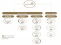 Overview of the Formation and Development Process of Vietcombank
 -
 General Overview of Promotions Aimed at Unfair Competition
 -
 General Overview of Tb 888 Trading Joint Stock Company.
- Experimental round 2: School year 2011 - 2012.
System
Class | Object | Symbol | Number of students | |
University | K13 Math | Experiment | TN 3 | 72 |
K13 Literature | Control | DC 3 | 84 | |
CD | K33 Math - IT | Experiment | TN 4 | 36 |
K33 English | Control | DC 4 | 33 |
The experimental and control classes are taught by the same teacher for the subjects: General Education (University) and General Education (College) according to the plan and program of the Department of Education compiled and approved by the school. The difference is that in the experimental class, the teacher teaches according to the experimental lesson plan , following the process of using BT in the types of lessons according to the model in section 3.2.3. In the control class, the teacher teaches according to traditional teaching methods, mainly presentations and lectures combined with some other teaching methods.
4.1.4. Experimental process
The experiment was conducted in the 2010-2011 and 2011-2012 school years at the College of Education and University of Education students of Hong Duc Thanh Hoa University. The experimental content is the BT system part 1: General issues of education . The purpose of this phase is to verify the effectiveness of the BT system built, on that basis to complete the BT system part: General issues of education .
Each experimental period we divide into 2 phases:
Phase 1 : Exploratory Experiment
This phase was conducted in the 2010-2011 school year at the Faculty of Natural Sciences and the Faculty of Foreign Languages. We observed teachers using teaching practice exercises in class ( theory, discussion) and students' attitudes when receiving learning tasks in each class and lesson . After finishing chapter I : "GDT is a science " , we gave students a test to assess their level of understanding and practical skills of the subject . ( Entrance test )
For self-study hours, this is a study hour that is mainly conducted outside of class hours, so we often evaluate the effectiveness of self-study hours through students' self-study notebooks. Teachers can ask students to research a specific content, then write a summary , research the study content of the following week or do exercises to practice practical skills , skills to handle situations in teaching and education. ( Refer to section 3.2.3)
Phase 2 : Impact experiment.
The experiment was conducted in the content of chapters II and III (Education and personality development, Purpose and tasks of education). After finishing chapter II, we gave students of the experimental and control classes (Test 2). Similarly, after finishing chapter III, we gave students of the experimental and control classes (Test 3) according to the teaching schedule of the detailed outline.
In each experimental phase, the experimental process includes the following steps:
* Experimental preparation : Includes:
- Experimental materials: Experimental class teaching plan, built GDH exercise system, reference materials are General GDH (College of Pedagogy textbooks by authors Nguyen Van Le, Nguyen Sinh Huy) and GDH (University of Pedagogy textbooks edited by author Tran Thi Tuyet Oanh) and some other reference materials, detailed subject outlines, spacious classrooms ensuring enough space for students to sit, with modern technical equipment that teachers can use in teaching when needed .
- Randomly select control class and experimental class, according to assignment
of the department.
- Selecting and training experimental lecturers: Before conducting the experiment, we selected enthusiastic and dedicated teachers with professional qualifications and experience. We discussed with the teachers to agree on the purpose and content of the experiment.
* Experimental implementation
- Provide students with detailed syllabuses and course reference materials, guide students in researching and performing learning tasks according to the schedule for each week of study, notify the number of regular and mid-term tests, test formats and schedules for each test, and check the preparation of conditions for organizing experiments.
- Test the initial level of students in TN and DC classes. Evaluate the initial results.
before the experiment.
- Conducting experiments : Teachers conduct experiments according to the established plan, using the built-in teaching practice system in experimental lessons. Researchers observe the experimental process with teachers, on that basis, exchange and draw experiences regularly during the experiment.
- Conduct a test of the results after organizing the experiment in the experimental class and the control class.
- Get feedback from TN class students.
* Processing experimental results :
To process the experimental results, first of all, the researcher needs to build standards and scales to evaluate the experimental results. Based on the results obtained between the experimental class and the control class, compare, evaluate the experimental results and draw conclusions.
4.1.5. Experimental standards and scales
To evaluate experimental results, we build standards and evaluation scales according to the following basic criteria:
* Assessment of students' level of knowledge acquisition : Through specific manifestations of students such as understanding the lesson, presenting the problem clearly and coherently, ensuring scientific and logical principles, and demonstrating creativity in problem solving. This criterion is demonstrated through a theoretical exercise in the test, we quantify it as follows:
Level 1 : Students have not determined the data and requirements of the exercise, do not know
problem solving orientation
Rating: weak (0 – 2.0 points).
Level 2 : Students identify the data and requirements of the exercise, however, the presentation of the problem is not clear, coherent, and the logical connection between the content of the exercise and the requirements to be achieved is not clear.
Rating: Poor (3.0 – 4.0 points).
Level 3 : Students can present the basic ideas of the exercise, however the results achieved are only at the level of reproducing knowledge, but not complete.
Rating: Average (5.0 – 6.0 points).
Level 4 : Students know how to present problems clearly, coherently and express them in personal language, know how to give illustrative examples, but the examples sometimes depend on the teacher's direction, and creativity in problem solving is not good.
Rating: Fair (7.0 – 8.0 points )
Level 5 : Students present scientific problems coherently and demonstrate creativity.
in problem solving, in accordance with practice.
Rating: Excellent (9.0 – 10.0 points)
* Assess students' attitudes in receiving and solving problems
To assess students' attitudes in performing exercises, we observed
student performance in class through the specific expressions below. Conclusions are drawn based on teacher assessment, student self-assessment, and group assessment .
TT
Symptoms | Level | ||||
Often through | Sometimes | Rarely | Never | ||
1 | Concentrate in class | ||||
2 | Actively participate in speaking in class | ||||
3 | Actively seek information to solve BT | ||||
4 | Active coordination between individuals in general activities | ||||
5 | Complete the learning tasks correctly plan | ||||
6 | Respect and listen to the opinions of teachers and friends | ||||
Tools for experimental assessment: Level of completion of scheduled tests , self-study notebooks, group discussion results (minutes of group discussion showing individual tasks and level of work completion), and sheets recording students' performances through observation of class hours.
* Assessing problem solving skills, testing skills, and evaluating results
Student performance is demonstrated through the following skills:
- Skill 1: Problem identification skills (Identify data and requirements of each exercise).
- Skill 2: Data screening skills , building hypotheses: based on determining the requirements of each exercise, screening the data, understanding the relationship between the data and the requirements of the exercise, the relationship between learned knowledge and the requirements of the exercise, discovering which data is basic and key to the exercise, reproducing the learned knowledge to build hypotheses and predict the solution direction of each exercise.
- Skill 3: Problem solving skills: A problem can have many different solutions, so based on judging the directions of solving the problem, students need to find the shortest and most correct way to solve the problem effectively. This is a very important skill, which has a great influence on the results of the student's work. To perform this skill well, students need to have qualities such as creative thinking ability, love for the job, perseverance and understanding of social practices.
- Skill 4: Skills to check and evaluate the results of the exercise: The process of solving exercises does not stop at finding a solution, but students need to have the skills to self-check and self-evaluate the results achieved compared to the requirements of the exercise. Performing this skill well not only brings new awareness, but also improves the thinking ability, the ability to analyze and synthesize problems of each student, fostering effective learning methods.
The proficiency of these skills is quantified into the following levels:
- Level 1 : Students cannot perform skill 1
Rating: weak (0 – 2.0 points)
- Level 2 : Students perform skill 1, but are still confused in filtering data, determining the relationship between data and the requirements of the exercise, and are not yet able to build a problem hypothesis.
Rating: Poor (3.0 – 4.0 points)
- Level 3 : Students perform skill 1 well, sometimes with confusion in skills 2 and 3.
Rating: average (5.0 – 6.0 points )
- Level 4 : Students perform skills 1,2,3,4 relatively completely but at a low level.
low proficiency in skills, poor creativity in problem solving
Rating: Fair (7.0 – 8.0 points).
- Level 5 : Students perform the operations completely, correctly, and proficiently, and are able to self-evaluate and determine the correct test results.
Evaluation: Excellent (9.0 – 10.0 points). The results of the evaluation of the proficiency of the skills are shown in the summary table below, the conclusion is drawn based on the evaluation of the lecturer and self-evaluation.
of students and test results.
TT
Skills | Levels | |||||
Level 1 | Level 2 | Level 3 | Level 4 | Level 5 | ||
1 | Identify the problem | |||||
2 | Data screening, building hypothesis building | |||||
3 | Problem Solving: | |||||
4 | Check and evaluate the results performance | |||||