If the sig value (β i ) is less than 0.05 => reject Ho. Thus, the i-th independent variable has an impact on the dependent variable. And the coefficient β i is greater or less than 0 will determine whether the independent variable has a positive or negative impact on the dependent variable.
- ANOVA and T-Test analysis
ANOVA and T-Test analysis to test the difference between groups of demographic factors (age, occupation, income, frequency, gender, marriage) according to factor i (where i is respectively tangible media, advertising, attitude, motivation, economy, subjective standards, intention to choose homestay as accommodation). With hypothesis H 0 : There is no difference between groups of demographic factors in factor i. With a significance level of 5%, any Sig value < 0.05 then conclude that there is a difference between groups of that demographic factor according to factor i.
The difference between ANOVA and T-Test is that with ANOVA the demographic factor has 3 or more groups, while T-Test has 2 groups.
CHAPTER 3 SUMMARY
After having the proposed model from the theoretical foundations and empirical models, the author conducts qualitative research through interviews with experts and focus group discussions to collect information, re-determine which factors affect the intention to choose homestay, and also considers what to remove, add or adjust in the observations such as changing words, clarifying the meaning of descriptive sentences, thereby adjusting the research model and related hypotheses to suit the Vietnamese market. Then the author completes the survey questionnaire and conducts the survey, synthesizes and encodes the data to run analysis in the software, the results will be presented in chapter 4.
CHAPTER 4: ANALYSIS OF RESEARCH RESULTS
4.1. Sample statistics
The author statistically describes demographic factors of gender, age, income, occupation, marriage, frequency to generalize and describe the research data as well as the surveyed subjects.
4.1.1. Gender
Table 4.1: Sample statistics by gender
Frequency (people) | Ratio (%) | |
Male | 187 | 57.7 |
Female | 137 | 42.3 |
Total | 324 | 100 |
Maybe you are interested!
-

 Cronbach's Alpha Reliability Coefficient of Components of the Scale of Factors Affecting Investment Capital Attraction for Tourism in Ba Ria Vung Tau Province
 -
 Cronbach'S Alpha of the Tourist Scenery Factor Scale Table 4.1: Reliability Assessment of the Tourist Scenery Scale
 -
 Reliability Testing Using Cronbach'S Alpha Coefficient
 -
 Testing of Scales – Cronbach'S Alpha Reliability Coefficient.
 -
 Testing the Reliability of the Scale Using Cronbach'S Alpha Coefficient
Source: Author analyzed and synthesized survey results (2018)
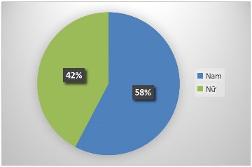
Figure 4.1: Sample statistics by gender
Source: Author analyzed and synthesized survey results (2018)
Based on the survey results in Table 4.1, we see that the proportion of men is higher than that of women, but overall this difference is not too much. Of the 324 survey subjects, 137 were women and 187 were men, with women accounting for 42.3% and men accounting for 57.7%.
4.1.2. Age
Table 4.2: Sample statistics by age
Frequency (people) | Ratio (%) | |
18 to 22 years old | 70 | 21.6 |
From 23 to 30 years old | 226 | 69.8 |
31 to 40 years old | 28 | 8.6 |
Total | 324 | 100 |
Source: Author analyzed and synthesized survey results (2018)
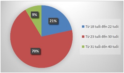
Figure 4.2: Sample statistics by age
Source: Author analyzed and synthesized survey results (2018)
Based on table 4.2, we see a clear age distribution, the majority of people surveyed are between the ages of 23 and 30, this is the age group with the highest proportion of 69.8%, specifically 226 people out of a total of 324 people surveyed, followed by the age group of 18 to 22 years old with 21.6% and finally the age group of 31 to 40 years old with 8.6%.
4.1.3. Marriage
Table 4.3: Sample statistics by marriage
Frequency (people) | Ratio (%) | |
No family | 221 | 68.2 |
Married | 103 | 31.8 |
Total | 324 | 100 |
Source: Author analyzed and synthesized survey results (2018)
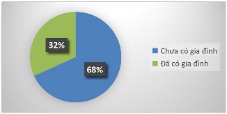
Figure 4.3: Sample statistics by marriage
Source: Author analyzed and synthesized survey results (2018) Table 4.3 clearly shows the difference between the two groups of single and married people. The single group has a rate twice as high as the married group, the group
The proportion of single people was 68.2%, and the proportion of married people was 31.8%.
4.1.4. Occupation
Table 4.4: Sample statistics by occupation
Frequency (people) | Ratio (%) | |
Student | 71 | 21.9 |
Office staff | 182 | 56.2 |
Manage | 49 | 15.1 |
Freelance business | 22 | 6.8 |
Total | 324 | 100 |
Source: Author analyzed and synthesized survey results (2018)
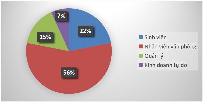
Figure 4.4: Sample statistics by occupation
Source: Author analyzed and synthesized survey results (2018)
According to the survey results in Table 4.4, the proportion between occupational groups has a significant difference. Specifically, the office worker group out of a total of 324 people surveyed has 182 people, accounting for the highest proportion with 56.2%, followed by the student occupational group with 71 people out of 324 people accounting for 21.9%, the management group with 49 people out of 324 people accounting for 15.1% and finally the self-employed group with 6.8%.
4.1.5. Income
Table 4.5: Sample statistics by income
Frequency (people) | Ratio (%) | |
Under 5 million | 44 | 13.6 |
From 5 million - <10 million | 141 | 43.5 |
From 10 million - <15 million | 75 | 23.1 |
From 15 million - <20 million | 41 | 12.7 |
From 20 million and up | 23 | 7.1 |
Total | 324 | 100 |
Source: Author analyzed and synthesized survey results (2018)
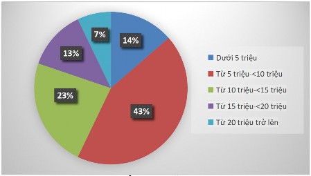
Figure 4.5: Sample statistics by income
Source: Author analyzed and synthesized survey results (2018). Survey results are shown in Table 4.5. The income of the surveyed group is mainly concentrated in the group from 5 to under 10 million, with 141 people out of a total of 324 people, accounting for 43.5%, followed by the group from 10 to under 15 million with 75.
The proportion of people is 23.1%, the groups under 5 million, from 15 to under 20 million and from 20 million and above are 44 people, 41 people, 23 people out of a total of 324 people, with proportions of 13.6%, 12.7% and 7.1% respectively.
4.1.6. Frequency
Table 4.6: Sample statistics by frequency
Frequency (people) | Ratio (%) | |
Seldom | 43 | 13.3 |
Sometimes | 133 | 41 |
Frequent | 111 | 34.3 |
Always | 37 | 11.4 |
Total | 324 | 100 |
Source: Author analyzed and synthesized survey results (2018)
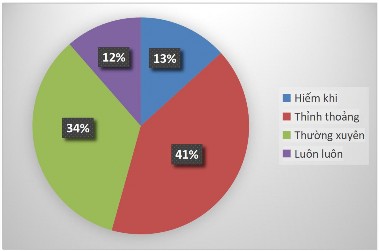
Figure 4.6: Sample statistics by frequency
Source: Author analyzed and synthesized survey results (2018) According to the survey results shown in Figure 4.6, the surveyed subjects occasionally chose homestay as a place to stay when traveling with 133 people out of a total of 324 people, accounting for 41%, the subjects who often chose homestay accounted for 34.3%, followed by the group of subjects who rarely chose homestay with 13.3% and the lowest
especially the group of people who always choose homestay with 11.4%.
4.2. Assessment of scale reliability
To evaluate the reliability of the scale, we remove the garbage variables and perform Cronbach's Alpha test for the scales of the independent variables and dependent variables in turn. After testing, the final result must satisfy the Cronbach's Alpha coefficient > 0.6, at the same time the measured variables must have a total adjusted correlation coefficient > 0.3, and when removing any variable, the Cronbach's Alpha coefficient will not increase, as well as there will be no duplication of variables, then the scale will achieve reliability and the observed variables are good measurement variables.
Table 4.7. Cronbach's Alpha reliability coefficient table of the scales after removing garbage variables
Encryption
Scale | Variable-total-difference correlation coefficient adjust | Cronbach's Alpha coefficient type variable | |
INDEPENDENT VARIABLE | |||
I. ATTITUDE | |||
Cronbach's Alpha = 0.828 | |||
TD1 | You think it would be fun to choose a homestay | 0.604 | 0.807 |
TD3 | You think it will be relaxing if you choose homestay | 0.645 | 0.788 |
TD4 | Do you think it would be beneficial to choose a homestay? | 0.699 | 0.763 |
TD5 | You feel that staying at a homestay is also very safe. | 0.674 | 0.775 |
II. SUBJECTIVE STANDARDS | |||
Cronbach's Alpha coefficient = 0.790 | |||
CQ2 | People important to you think you should choose a homestay | 0.657 | 0.688 |
CQ3 | People whose opinions you value agree with your choice of homestay. | 0.627 | 0.723 |
CQ4 | You see most people around you have stayed at a homestay. | 0.615 | 0.734 |
III. MOTIVATION | |||
Cronbach's Alpha = 0.786 | |||
DL1 | Choosing a homestay will give you the experience a different way of life (eating and living with local people) | 0.515 | 0.771 |
DL2
Choosing a homestay will help you understand the culture at the tourist destination. | 0.646 | 0.712 | |
DL4 | Choosing a homestay will help you visit many unique beautiful scenes. | 0.511 | 0.773 |
DL5 | Choosing a homestay will allow you to enjoy local specialties. | 0.735 | 0.664 |
IV. TANGIBLE MEANS | |||
Cronbach's Alpha = 0.841 | |||
HH1 | Full facilities and equipment, convenient | 0.654 | 0.806 |
HH2 | The rooms in the homestay are clean. | 0.591 | 0.822 |
HH3 | Convenient transportation (easy to travel, available) rent means of transport such as bicycles, motorbikes) | 0.659 | 0.806 |
HH4 | The homeowner always keeps everything neat and tidy in the common living spaces between the owners. home and visitors | 0.622 | 0.815 |
HH5 | Beautiful natural landscape environment | 0.703 | 0.792 |
V. ECONOMIC CALCULATION | |||
Cronbach's Alpha = 0.787 | |||
KT1 | Accommodation at reasonable prices | 0.657 | 0.707 |
KT2 | Price matches quality of service | 0.537 | 0.763 |
KT4 | Perceived value is higher than cost | 0.601 | 0.731 |
KT5 | Homestay is cheaper than hotel | 0.590 | 0.736 |
VI. ADVERTISING | |||
Cronbach's Alpha = 0.862 | |||
QC1 | You often see homestay advertisements on social networks. | 0.631 | 0.86 |
QC2 | You often see homestay introductions on electronic newspapers. | 0.775 | 0.798 |
QC3 | You often see homestay reviews on travel forums. | 0.760 | 0.807 |
QC4 | You see homestay on reputable online booking websites | 0.688 | 0.833 |
DEPENDENT VARIABLE | |||
INTENTION OF CHOOSING HOMESTAY AS A PLACE TO STAY | |||
Cronbach's Alpha = 0.818 | |||
YD1 | You will choose homestay as your accommodation when traveling | 0.677 | 0.743 |