Create Conditional Ranges for Use with Database Functions

LESSON 4

CHART WIZARD

In addition to using two-dimensional arrays to organize data, in Excel to show the correlation between data series we can represent them by charts. Charts are in the form of graphics, divided into many types: Area (area type); Bar (bar); Column (column); Line (line); Pie (circular arc containing angle); XY-Scatter (discrete point)... These types can be represented in 2-dimensional (2-D) or 3-dimensional (3-D).

4.1. Components of the chart

+ Data area : a continuous or discrete range of spreadsheet cells selected to be used as data for the chart, which can be organized in rows or columns called a series .

data. Each cell constitutes a data point.

data on chart

and marked

(markers) by different symbols. The data area can consist of a row (or column) containing labels.

+ Coordinate axes : a system of vertical or horizontal lines that determine the scale of data points , with tick marks on the axes. There are usually two types of axes: category axes and value axes.

+ Legend box : contains symbols representing the data series present in the chart. The legend can be placed at any position in the chart .

+ Title : text line that labels the chart and axes .

Sample chart

Food Gas Motel

Jan Feb Mar Apr May Jun

4.2.Using the Chart Wizard

Ÿ Step 1: Select the data area containing the chart data. You can select continuously or

Discrete groups cells by rows or columns.

Ÿ Step 2: Click on the Chart Wizard icon or select [Insert]Chart. When the cursor

in the form of a plus sign (+), we draw a rectangular frame that defines the initial size and position of the chart. Note: you can choose to draw on the sheet containing the data or on another sheet.

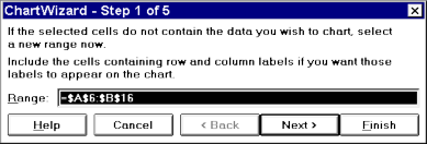
Ÿ Step 3: The data area selection box appears:

Since the data area has been selected in step 1, we choose [Next] to go to the next step (choose the chart type), or choose [Finish] to finish (use the default chart format), and can create a new format later. If the data area appears here incorrectly, we can use the mouse to select another area.

Ÿ Step 4: Select a chart type and select a subtype of it

For example, the Column type has the following forms:

Ÿ Step 5: Provide additional information, such as:

- Data Series in Rows/Columns

- If the data area contains labels, specify the row or column numbers to label the axes at the [x] and [y] values, otherwise enter 0 for these values:

Use First [ x ] Row(s) for Category (X) Axis Labels Use First [ y ] Column(s) for Series(Y) Axis Labels

- Option to add a Legend to the chart

- Enter a title for the chart and titles for the axes.

4.3. Edit and create chart shapes

After selecting [Finish], a chart will appear in the rectangular area that we defined in step 2. We can continue to adjust, shape, add/remove chart components. To do this, just D-click on the appropriate areas and adjust the information in the corresponding dialog boxes. For example, we can change components such as: size, color, font, remove grid lines, modify or add data; change the chart style to the appropriate form...

 In Excel-97 (or 2k3), the chart creation tool is simpler. Users do not need to draw the area that will contain the chart in advance (in Step 2) because Excel will automatically create it. In addition, Excel-97 also adds many types of charts. Below are the dialog boxes of the Chart Wizard in Excel-97:

* Step 1(of 4 steps): select Chart type

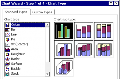
- In this step, we select a main chart type and then select an appropriate type from its set of subtypes. The figure below illustrates the Column type and its subtypes.

* Step 2 : Specify the data source to use in the Chart

- Note here that if before executing the chart creation command, we have selected or are in the data area, Excel will automatically mark the data area.

- Usually Excel correctly analyzes the data value series by column (Series in

Columns) or Series in Rows, if necessary we can re-specify this value.

* Step 3 : Add options

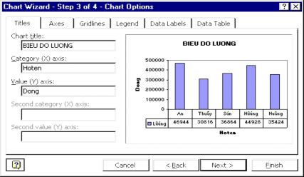
- In this step, there are many options for us to change and add components to the chart as required.

* Step 4 : Choose the chart location

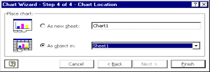
- Here we can specify the position of the chart in existing Sheets or create another Sheet to contain the chart.

 After clicking Finish we have the following result:

500000

400000

300000

200000

100000

THE FUTURE

Thuong

Sun Huong Huong

* We can easily edit elements in the chart by D-clicking on the position that needs to be affected.

* Introducing chart creation tools:

LESSON 5

DATABASE IN EXCEL

5.1. Concept of database (Data Base)

Database (also known as data table) is a structured collection of interrelated information, organized according to a certain principle to reflect the properties of an object class. There are database organization models such as: hierarchical model; network model; relational model...

In which, the relational model can be represented by a 2-dimensional array, organized

into rows and columns. Each row contains information about an object, called a record, each column contains information reflecting common properties of the objects, called a field.

In Excel, databases are organized in the relational model as lists. A list is a special type of spreadsheet, consisting of a continuous range of cells. In a list, the first row contains the names of the columns, and the remaining rows contain data about the objects in the list.

5.2. Instructions for creating a list in Excel

Microsoft Excel provides many convenient functions for managing and analyzing data in a list. To take advantage of these functions, enter data in the list according to the following suggestions:

Ÿ About size and location

- There should not be more than one list in a worksheet.

- It is recommended to leave at least one blank row and column separating the list from the spreadsheet data. This makes it easier for Excel to automatically recognize which list to work with.

- Do not leave rows with no data in the list.

- Avoid placing important data on the left or right of the list, as the data may be hidden when filtering the list.

Ÿ About column labels:

- It's a good idea to create column labels in the first row of your list. Excel uses labels to create reports, search, and organize data.

- Use font formatting, alignment... for column labels that are different from the data in the list. Use borders around the cells of the labels in the first row to separate them from the data area.

Ÿ About content:

- Design the list so that all rows have similar items in the same column.

- Avoid adding spaces at the beginning of cells, as this affects sorting and searching.

- Do not use blank rows to separate column labels from data.

Ÿ Name:

- You should name the list to make it easier to act on the list (such as calculating, filtering information...)

- When selecting the data area of the list to name, be sure to select the first row in the list containing the column labels.

5.3.DB functions

Excel provides many functions for working with list-based databases. These functions all have the same syntax structure, but differ in functionality.

1. General structure of the DB function

Dfunction(database,field,criteria)

- Function names start with the character DSUM)

D, followed by names like

SUM, MIN,... (for example:

- database is an Excel list database, usually a predefined name of the list to be affected.

- field is the column label name enclosed in double quotes or the column number in the list (counting from column 1) or the reference name of the column label that will be affected by the function (for example, calculating on a column of the list).

- criteria is the condition area that defines the necessary conditions that the function must satisfy to act on the data field specified by field.

Ÿ Function: The DB function acts on the data field (filed) of the list.

(database) according to the conditions specified by the criteria field .

2. Create a conditional range for use with database functions

Criteria is a reference to a range of cells that contains specific conditions for the function. The DBMS function returns a calculation on a column of the list that matches the constraints specified by the criteria range. The criteria range usually contains a column label that represents the values in the columns that participate in the condition. The reference to the criteria range can be entered into the function as a range of cells or through the name assigned to the range of cells.

Ÿ General form of the conditional area:

Field name (column label)

WAGE

For example:

condition

>= 525000

In the cell containing the condition, you can use the relational operators: >, <, >=, <=, <>, = or the wildcard characters ?, * similar to those in the MS-DOS operating system (for example, the condition X* means that the string data starts with X, the remaining characters are optional). To find exact string values, we use the form: = “=string_value”. Note that the results of the string functions (Left, Right, Mid) are string types.

The criteria area can contain multiple Field Name cells, and multiple criteria can be placed on the same row or in different rows. Criteria placed on the same row have the meaning of the AND operator; criteria placed on multiple rows have the meaning of OR.

For example:

WAGE

WAGE
>= 350000	<= 500000

Maybe you are interested!

Means SALARY >= 350000 and (AND) SALARY <= 500000

WAGE

TDVH
>= 350000	University
<=250000

Means SALARY >=350000 and (AND) TĐVH is University or (OR) SALARY

<= 250000 and TDVH is any (because the corresponding cell does not contain a condition value).

F Note: The criteria range can be organized in the first rows of the spreadsheet, and can be hidden later without affecting the data in the spreadsheet. Or it can be organized in a different sheet than the sheet containing the list.

3. Introduce some common Excel database functions

1. DSUM (database, fields, criteria)

The DSUM function calculates the sum of a field column in the database according to the specified criteria.

out by

For example, in a salary list, you can sum the condition column Basic Salary or by Education Level...

2. DMAX , DMIN , DAVERAGE

Total Salary by

These functions return the maximum (max), minimum (min), average (average) value of a data column (field) in a list according to the specified criteria.

3. DCOUNT (database, [field,] criteria)

DCOUNTA (database, [field,] criteria)

The DCOUNT function counts the number of cells containing numeric values; DCOUNTA counts non-blank cells (i.e. cells containing data) in a column of a list that match the conditions specified by the criteria range. The special thing here is that the [filed,] argument can be omitted, then these two functions will count in all records (rows) of the list.

4. Example of the DB function

Suppose we have the following data list (from B2 to D7 - see illustration table)

We can calculate the total of the TONG column under the condition that the item is of type GAO, as follows:

or or

=DSUM(B2:D7, “ TONG ”, B25:B26) (enter field name)

= DSUM(DATA10, 3 , B25:B26) (column number)

= DSUM(DATA10, D2 , CRT10) (cell number)

(Where DATA10 is the name of the data list; CRT10 is the name of the condition range B25:B26)