LIST OF REFERENCES
Vietnamese Document Catalog
1. Do Le, 2013. Restructuring the system of credit institutions: Many positive results have been achieved. http://vietstock.vn/2013/04/tai-cau-truc-he-thong-cac-tctd-da-dat- nhieu-ket-qua-tich-cuc-757-290502.htm .
2. Ho Tuan Vu, 2011. The benefits and limitations of bank mergers and acquisitions. Auditing Journal No. 9/2011.
3. KPMG, 2014. Vietnam Banking Industry Survey 2013
4. Le My, 2012. HBB merges with SHB, who benefits? Business Forum. http://dddn.com.vn/tai-chinh-ngan-hang/habubank-sap-nhap-vao-shb-ai- loi--20120406092358145.htm
5. Minh Duc, 2013. SHB General Director looks back at the Habubank merger . http://vneconomy.vn/doanh-nhan/tong-giam-doc-shb-nhin-lai-vu-sap-nhap-habubank-20130828033218856.htm
6. Ngo Dang Thanh, 2010. Evaluation of resource utilization efficiency of some commercial banks in Vietnam applying data envelopment method (DEA).
7. State Bank of Vietnam, 2013. Circular No. 02/2013/TT-NHNN Regulations on classification of assets, provision levels, methods of setting up risk provisions and use of provisions to handle risks in the operations of credit institutions and foreign bank branches.
8. State Bank of Vietnam, 2014. Circular 36/2014/TT – SBV Regulating limits and guarantee ratios in the operations of credit institutions and foreign bank branches.
9. An Binh Commercial Joint Stock Bank (ABB), 2008 – 2014. Financial report
10. Hanoi Housing Commercial Joint Stock Bank (HBB), 2008 – 2011. Financial report
11. National Commercial Joint Stock Bank (NVB), 2008 – 2014. Financial report
12. Saigon – Hanoi Commercial Joint Stock Bank (SHB), 2008 – 2014. Financial report
13. Saigon – Hanoi Commercial Joint Stock Bank (SHB), 2008 – 2014. Annual report
14. Saigon - Hanoi Commercial Joint Stock Bank, 2012. Summary of the Bank's charter after the merger
15. Saigon – Hanoi Commercial Joint Stock Bank, 2012. Summary of merger contract
16. Saigon – Hanoi Commercial Joint Stock Bank, 2012. Summary of merger project
17. Vietnam Prosperity Joint Stock Commercial Bank, 2008 – 2014. Financial report
18. Peter S. Rose, 2004. Commercial Bank Management. National Economics University Publishing House, Hanoi
19. Vietnam Chamber of Commerce and Industry (VCCI), 2012. Vietnam Credit Index Annual Report 2012
20. National Assembly, 2010. Law on credit institutions. Phuong Dong Publishing House.
21. Prime Minister, 2006. Decision 112/2006/QD – TTg on approving the Project on development of Vietnam's banking industry to 2010 and orientation to 2020.
22. Prime Minister, 2012. Project "Restructuring the system of credit institutions in the period 2011 - 2015".
23. Tran Huy Hoang, 2012. Commercial Bank Management . Ho Chi Minh City Economic Publishing House.
English Document Catalog
1. Aziz P., M., and Lennart, H., 2002. Measurement of inputs and outputs in the banking industry . Tanzanet Journal, 3 (1): 12 – 22.
2. Charnes, A., W. W. Cooper, and E. Rhodes,1978. Measuring the Efficiency of Decision Making Units . European Journal of Operational Research, 2: 429- 444
3. Coelli, T., 1996. A guide to DEAP version 2.1: A data envelopment analysis (computer) program . CEPA Working paper 96/08, University of New England, http://www.une.edu.au/econometrics/cepawp.htm .
4. Coelli, T., Rao., DS and GE Battese, 1996. An Introduction to efficiency and productivity analysis . Boston, MA: Kluwer Academic Punlishers.
5. Farrell, M., 1957. The measurement of productive efficiency. Journal of the Royal Statistical Society . Series A 9 (General), 120: 253 – 290.
6. International Monetary Fund (IMF), 2006. Financial Soundness Indicators (FSIs) Complilation Guide .
7. Neena Sinha, Kaushik and Timcy Chaudhary, 2010. Measuring Post Merger and Acquisition Performance: an investigation of selected financial sector organizations in India . International Journal of Economics and Finance, Vol.2, No.4, pages 190 – 200.
8. Sherman, HD, F. Gold, 1983. Evaluating operating efficiency of service business with data envelopment analysis – empirical study of bank branch operation . Working paper 1444 – 83, Massachusetts Institute of Technology.
9. Tze San Ong, Cia Ling Teo and Boon Heng The, 2011. Analysis on financial performance and efficiency changes of Malaysian Commercial Banks after mergers and acquisitions . International Journal of business and management tomorrow, vol.1, No.2 : 1 – 16
10. Wirnkar, A.D., and Tanko, M., 2008.CAMEL(S) and Bank Performance evaluation: The way forward. Http://ssrn.com/abstract=1150968
Appendix 1: Input – oriented measures
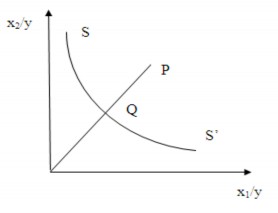
Farrell illustrates his idea of technical efficiency using a simple example of firms using two inputs (x 1 and x 2 ) to produce one output (y) under constant returns to scale. Firms lying on the perfectly efficient isoquant, depicted by the curve SS' in the graph, allow for a measure of technical efficiency.
Technical efficiency by input approach
O
If firms use the inputs at point P to produce an output, then the firm's technical inefficiency is defined by the gap QP. This is the amount by which all inputs can be reduced without reducing output. This level of inefficiency is usually expressed as a percentage and is expressed as the ratio QP/OP. The firm's technical efficiency TE is measured by the ratio TE 1 = OQ/OP = 1 – QP/OP and ranges from 0 to 1. In this example, point Q is technically efficient because it lies on the efficiency isoquant.
This measure of efficiency assumes that the firm's production function is perfectly efficient, which is known. In practice, it is impossible to know the efficiency isoquant. Therefore, the efficiency isoquant must be estimated from sample data.
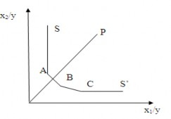
Farrell (1957) suggested using a non-parametric piecewise convex isoquant such that the observation points do not lie to the left or below it. And following this suggestion of Farrell, Charnes, Cooper and Rhodes (1978) developed the DEA model. The input minimizing DEA model is illustrated as follows:
O
Enterprises A, B and C are completely relatively efficient compared to other enterprises in the same research sample, so they are on the efficiency frontier. Enterprise P is not completely relatively efficient, so it is not on the efficiency frontier.
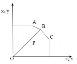
Appendix 2: Output – oriented measures
Output-oriented efficiency is the opposite of input-oriented efficiency. The difference between input-oriented and output-oriented efficiency is illustrated using a simple example of an output and an input as shown in Figures 1.3 and 1.4. According to Figure 1.3, under decreasing returns to scale, technical efficiency is represented by the function f(x) and the firm is inefficient at point P. Input-oriented technical efficiency is measured by the ratio AB/AP, while output-oriented technical efficiency is measured by the ratio CP/CD. The graph shows that these two ratios are different. According to Figure 3b, under constant returns to scale, input-oriented and output-oriented technical efficiency are equivalent.
f(x)
f(x)
O

Technical efficiency under conditions of variable output with scale Technical efficiency under conditions of constant output with scale
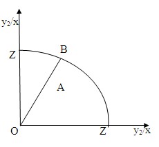
We can consider measuring technical efficiency in terms of the output bias for the two-output and one-input case. In the constant-return-to-scale case, technical efficiency can be calculated based on the unit production possibilities curve in two dimensions:
Technical efficiency based on production possibilities curve
Z'
The ZZ' curve is the unit production possibilities curve and point A is considered to be the inefficient point. The inefficient point A lies below the curve in this case because ZZ' represents the upper limit of the production possibilities frontier.
The output-oriented measure of efficiency can be defined as follows: The gap AB represents technical inefficiency. Therefore, it is the proportion of output that can be increased without requiring additional inputs. Then TE 0 = OA/OB. The output-maximizing DEA model is illustrated similarly to the input-minimizing DEA model.
DEA model maximizes output
Appendix 3: Graph depicting CRS and VRS boundaries
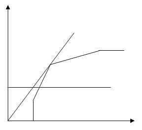
y
CRS
VRS
P C
AP
PV
O
x
Appendix 4: Performance evaluation criteria system according to CAMEL model
STT
Indicator name | Recipe | Meaning | Evaluation standards | Source | |
1. | Capital Aquadecy – Equity | ||||
1.1 | VTC level 1 coefficient | yes
| Level 1 VTC Proportion – VTC with high stability in total VTC | ≥ 50% | |
1.2. | Level 2 VTC coefficient | yes
| VTC ratio level 2 in total VTC | ≤ 50% | |
1.3. | Capital Adequacy Ratio - CAR |
compost | VTC's guarantee of value TSC risk conversion | ≥ 9% | Circular 36 |
1.4. | Financial leverage ratio | burp
| The degree of financial leverage (debt leverage) used. Represents risk. financial risk of the bank. | ||
1.5. | Internal Capital Generation Ratio | yes
yes | The ability to generate capital from the bank's own operations, demonstrating self-financing ability of NH from retained earnings | ||
1.6. | Fixed Asset Investment Ratio on Equity | e a D
| The level of VCSH funding for with fixed asset investment activities | ≤ 50% | Law of TCTD 2010 |
1.7. | Financial investment ratio on equity | what
| The level of VCSH funding for with financial investment activities | ||
1.8. | Capital contribution and share purchase ratio | oh my god
| The level of VCSH funding for operations contribute capital, buy shares | ≤ 40% | Law on Credit Institutions 2010 |
2. | Asset Quality – Asset Quality | ||||
2.1. | Loan/investment/fixed asset structure in TTS |
Head
D
| Represents the allocation between asset classes, reasonable allocation will help increase profitability. profit, risk reduction | ||


Maybe you are interested!
-
 Improving business efficiency of Vietnam Technological and Commercial Joint Stock Bank - 2
 -
 Objectives and Operational Directions of Saigon - Hanoi Commercial Joint Stock Bank Shb
 -
 Current Business Performance of Vietnam Joint Stock Commercial Bank for Investment and Development
 -
 Improving the quality of customer care services at Saigon Thuong Tin Commercial Joint Stock Bank - Hue Branch - 11
 -
 Improving business efficiency of Vietnam Technological and Commercial Joint Stock Bank - 4