Var Values of Normal Distribution and Thick Tailed Distribution

The conditional copula method (using only copula-Student) is used to estimate the VaR of a portfolio constructed from the returns of two stocks REE and SAM with equal weights. The post-test results show that the VaR estimation result using the GARCH-copula-T method is superior to the two Riskmetric methods and the unbiased estimation method.

Recently, in the article “Multidimensional copula and its application in risk measurement”, the authors Tran Trong Nguyen and Nguyen Thu Thuy ([17]) applied the conditional copula method (with 2 types of copula-Gauss and copula-T) to calculate the VaR of a portfolio of 4 stocks FPT, STB, REE, SAM with equal weights. The post-test results showed that the GARCH-copula-T model is more suitable than the GARCH-copula-Gauss model. However, in this study, the authors have not compared the GARCH-copula method with other methods.

Thus, in Vietnam, there have been initial studies approaching EVT and the copula method to measure risk. However, these are still quite new approaches in quantitative risk management research in the Vietnamese financial market. According to these approaches, we can continue to research the Vietnamese financial market from many perspectives:

- First , we need to conduct additional empirical analysis of other copulas and rely on testing criteria to select the copula that fits the actual data better. If possible, we should add more synthetic copulas to better describe the dependence structure of the series because in reality, systemic risk can be of many types.

Maybe you are interested!

- Second , we need to consider the time variation of the copula over the entire cycle of the sample, that is, to study dynamic copula models. This variation is usually studied in two forms: The first form is that over the entire cycle we consider a family of copulas but the parameters of the copula vary, and therefore we need to choose equations to describe the time variation of the parameters of this copula; The second form is that over different stages of the entire cycle, we use different copulas.

- Third, we can approach the methods: Copula-Vine method, factor copula,.. to build more multidimensional copula families, to better describe the dependency structure of many assets.

- Fourth, measure the dependence of extreme values of assets, that is, measure the dependence of assets when the market fluctuates abnormally. At the same time, we need to study EVT for multi-dimensional cases, to describe simultaneous extreme events for multi-asset portfolios.

- Fifth, study the optimal investment portfolio based on risk measures VaR and ES.

Furthermore, applied studies of the ES model for multi-asset portfolios are almost non-existent in the Vietnamese stock market, so studying this model to predict portfolio losses in bad market conditions is necessary.

Through that, we can see that in the trend of world integration, in Vietnam, there have been initial studies on quantitative risk management with different approaches, but they are still very limited in both theoretical and empirical aspects. The thesis will study some risk measurement models in the Vietnamese stock market with new approaches to hope to have better results in risk management in the Vietnamese stock market.

In the next part, we will focus on studying in more detail some risk measurement models: GARCH model, CAPM model, VaR model, ES model. While studying these risk measurement models, we often use directly with the return series of assets or the return of portfolios for research. We

have yield of assets

r  P t  P t  1 , where

P t  1

P t , P t  1

is the price of the asset at time t, t-

1. So at time t-1 then

P t  1

known, so to measure the risk of an asset we need

risk assessment of yield

r t . When the yield calculation period is short (trading days), the profit

The yield is quite small, so people often approximate the asset yield by the logarithm of the yield.

( r  ln  P t  ); with the logarithmic yield calculation, the advantage is that it can be linearized

t P 

t  1 

especially when calculating for multiple cycles.

1.3. Some risk measurement models

1.3.1. Volatility measurement model

Univariate GARCH model

Suppose we consider a yield series  r t has the condition:  r t/ t 1 , with

r t log( P t/ P t 1 ) ,

and  t − 1 is the information set related to r t

obtained up to time t -1.

The ARMA(m,n) model describes the average return ([9, p.675]) and the GARCH(p,q) model describes the variance ([9, p.688-689]).

 Average equation

r t  t u t ,

 t  0   i r t  i    i u t  i

(1.5)

i  1 i  1

 Variance equation

u t t  t ,  t

are independent random variables with the same distribution,

2  u 2 2

(1.6)

t 0

i  1

it  ist  ss  1



 0  0;  1 ,..., p  0;  1 ,...,  q  0 ;

max( p , q ) i  1

(  i   i )  1 .

If p>q then

 s  0 for s>q , if p<q then  i  0 for i>p .

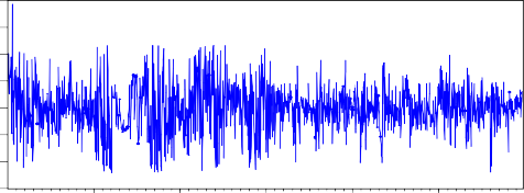
We have a graph illustrating the series with variable error variance as shown in Figure 1.3. On the graph in Figure 1.3, we see that there are periods when the yield series of the VNINDEX index fluctuates greatly and has a high concentration level, however, there are periods when the VNINDEX yield series fluctuates with a smaller amplitude. Based on the characteristics of the yield series

The VNINDEX index helps us identify that this is a series with variable variance.

The new univariate GARCH model only models and measures the conditional variance for each return series.

.08

.06

.04

.02

.00

-.02

-.04

-.06

250 500 750 1000 1250

RVNINDEX

Figure 1.3. VNINDEX index yield series graph

(Source: author draws from aggregated data of VNINDEX yield series ([50]))

But when studying issues such as portfolio risk, optimal portfolio selection, etc., we need to analyze the dependence of return series on each other. This is a very important issue in economic research, the multivariate GARCH model gives us an approach to solve the above problem.

Multivariate GARCH model

Generalized multivariate GARCH model

Consider the yield vector: r t  ( r 1 t , r 2 t ,..., r Nt ) ' , where r it is the yield of the i-th asset at

time t ,

r it  log( Pi , t / Pi , t  1 ) . The multivariate GARCH model has the form ([30, p. 6] ) :

in there:

is the parameter vector,

r t   t ( )  u t , u t  H 2 ( ) z t , (1.7)

 t ( )

is the average of r t

corresponding to parameter ,

H t ( ) is the variance matrix of r t

corresponding to parameter ,

z t - are independent random variables with the same probability distribution,

Var ( z t )  I N .

E ( z t )  0 and

We have the variance matrix ([30, p. 6]):

1 1

V ar( r t |  t  1 )  V ar( u t |  t  1 )  H 2 V ar( z t |  t  1 )( H 2 ) '  H t , (1.8)

 t  1 is the information available up to time t-1.

Depending on the specific analysis of the matrix

H t ( )

we have models

Specific multivariate GARCH ([30]): VEC model, BEKK model, DCC model,…

 Model estimation: To estimate a univariate GARCH model or a multivariate GARCH model, we often use the following methods: Maximum Likelihood (ML) method, Quasi-maximum likelihood (QML) method ([9], [30]).

 Model testing: When applying the model, we must test the model's suitability with a number of testing procedures ([9], [30]): Stationarity testing, autocorrelation testing, distribution type testing, etc.

1.3.2. CAPM model

The CAPM model describes the relationship between risk and expected return ([3, p. 214]):

in there:

E ( r i ) r f r i is the return on asset i. r f is the risk-free rate.

  i E ( r M  r f )

, (1.9)

r M is the return on the market portfolio.

Beta is a measure of the volatility or systematic risk of a security or portfolio relative to the market as a whole. The beta of an asset (or portfolio) provides information that helps us determine the riskiness of the asset, determine the risk premium of the asset, and other

information for the fair pricing of risky assets; beta is typically estimated using a linear regression model.

When applying the CAPM model, we also need assumptions ([3]): assumptions about investors, assumptions about the market and assets in the market. Up to now, there are still many controversies about the practical applicability of CAPM, however, the CAPM model still creates a turning point in the research and analysis of financial markets.

1.3.3. VaR model

The risk value of an asset portfolio represents the level of loss that can occur to the portfolio or asset in a period k (time unit) with a confidence level of (1- α)100%, denoted as VaR ( k , ).) , and is defined as follows ([3, p. 188]):

P ( X 

VaR ( k , ))  

(1.10)

where X is the k-period profit-loss function of the portfolio, 0   1 .

Thus, if the investor holds the portfolio after k periods, with confidence (1  ) 100%, the probability of losing an amount will be equal to | VaR ( k , ) | under normal market conditions.

VaR model is one of the models to measure the market risk of assets and portfolios. Using VaR model to measure and warn early about the loss in value of the portfolio when the price of each asset in the portfolio fluctuates; it helps investors estimate the level of loss and implement risk hedging.

As we know, the VaR model is quite popular in managing market risk and credit risk of portfolios. However, VaR does not satisfy property 2 of strict risk measurement ([4], [33]) (it only satisfies when the portfolio has a normal distribution), so the diversification rule in investment is broken. We have a new approach in measuring portfolio risk through the use of the Expected Loss measure.

1.3.4. ES Model

After calculating the VaR of the portfolio, we are interested in cases where the actual loss of the portfolio exceeds the VaR threshold and calculate the average (expected) of

these loss levels ([4], [33]). We have the following concept:

The expected loss of the portfolio with confidence level (1- α)100%, denoted by ES(α), is the conditional expectation ([4, p. 7]):

ES ( )  ES  E ( X / X  VaR ( )) . (1.11)

VaR(95%

ES(95%)

Thanks to some superior properties over VaR, the use of ES risk measure represents a more complete risk measurement than using VaR. We have a graph illustrating the VaR and ES values of asset returns in Figure 1.4. Thus, when we have information about the probability distribution of asset returns, we can determine VaR and ES. Moreover, the VaR and ES values will depend on the left tail (describing the loss) of the probability density function of asset returns.

Figure 1.4. VaR and ES values of asset returns

(Source: The author of the thesis refers to [3, p.190])

VaR(95%)

Figure 1.5. VaR values of normal distribution and thick tail distribution

(Source: Author's drawing to illustrate normal distribution and thick-tailed distribution)

In Figure 1.5, we have the density function graph of the normal distribution (N) and the density function graph of the distribution with a thicker tail (F) than the normal distribution. Thus, with the same 95% confidence level, the VaR value (95%) (in terms of magnitude) corresponding to the normal distribution will be smaller than the VaR value (95%) corresponding to the distribution with a thicker tail.

Furthermore, the ES measure has several properties ([4], [33]):

 ES is a measure of the portfolio's coherent risk.

 Any other rigorous risk measure g(X) of the portfolio can be expressed as a convex combination of ES and ES  g(X).

Thus, the determination and calculation of ES of a portfolio has both replaced VaR in the role of a more complete risk measurement and shown that this is a superior risk measure. The ES measure has only recently been proposed as a supplementary risk measure to VaR, but its significance and importance in financial risk management are very clear. However, due to its more complex structure than VaR, to calculate and estimate ES, it is necessary to develop appropriate methods, especially when we refer to portfolios with complex structures such as portfolios of financial and credit institutions. Next, we study the methods of estimating VaR and ES models.

1.3.5. Methods of estimating VaR and ES models

Typically, we have two main methods of estimating VaR and ES: parametric and non-parametric methods.

1.3.5.1. Parametric method

This method is based on the assumption of the distribution of the return r : for example, normal distribution, Student distribution, generalized Pareto distribution, etc. Then from the past data of r , we use estimation methods in statistics and econometrics (maximum likelihood, generalized moment, ARCH, GARCH, etc.) to estimate the characteristic parameters of the distribution and derive the corresponding estimates of VaR and ES ([4], [19]).

Below, we have the formula to estimate VaR, ES for 2 cases:

Comment